One Mathematical Model of Modern Monetary Operations
I confess immediately that I chose the title and subtitle for this post because their acronyms are palindromes.
The subtitle is more accurate than the title, because this model considers only the monetary aspects of MMT: the Job Guarantee and inflation management components are not yet incorporated. But the monetary assertions of MMT remain in dispute in economic and political circles, so it is worth putting these into a mathematical model where their veracity can be tested.
The primary stimulus for developing the model was the publication of Stephanie Kelton’s The Deficit Myth. Stephanie has written the book for non-technical readers, and she’s done a very good job: it’s a very easy read that explains why many conventional wisdoms about government spending are wrong. But MMT is facing heavy resistance in political and economic circles, with my favourite to date being a motion before the US Congress, posted by Representative Kevin Hern, to resolve:
That the House of Representatives (1) realizes that deficits are unsustainable, irresponsible, and dangerous; and (2) recognizes— (A) that the implementation of Modern Monetary Theory would lead to higher deficits and higher inflation; and (B) the duty of the House of Representatives to condemn Modern Monetary Theory.
The objective of this series of posts is to allow the assessment of the first part of this motion—the assertion that “deficits are unsustainable, irresponsible, and dangerous”.
The models in this post are built in the Open Source system dynamics program Minsky, whose unique feature is the capacity to build models of financial flows using what are called Godley Tables (in honour of Wynne Godley, the pioneer of stock-flow-consistent-modelling). These tables enforce the “law of accounting” that (see Figure 1).
Figure 1: A blank Godley Table
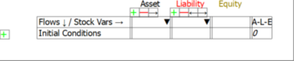
Once an account is flagged as an “Asset” for one entity, Minsky knows that it has to also be shown as a “Liability” for another entity. This
makes it possible to take an integrated look at the financial system, which allows us to assess Hern’s motion from the perspective of the entire monetary system, and not just the Government’s view of it.
An Integrated View of Deficits, Surpluses, and Equity
This Minsky model is a simple but complete model of a domestic monetary system. It has six sectors which can be divided into five components:
- The Treasury, and the Central Bank, which together constitute the Government Sector;
- The Banking Sector;
- The Firm Sector, Capitalists and Workers, which constitute the “NonBank Private Sector“;
- The NonBank Private Sector and the Banking Sector, which constitute the “NonGovernment Sector“; and
- The sum of the Government and the NonBank Private Sector, which constitute the “NonBank Sector“.
For simplicity, taxes—and government spending—are levied only on the Firm Sector, and banks make loans only to firms (the aggregate outcome would be the same if the model were generalized to have taxes and spending and loans in all sectors—it would just be much harder to read the tables).
There are just thirteen financial flows:
- Treasury spends on firms (Spend);
- Treasury taxes firms (Tax);
- Treasury sells bonds to the Banking Sector to cover any deficit (BondB);
- Treasury pays interest on Treasury Bonds owned by the Banking Sector (InterestBonds);
- The Central Bank buys and sells Treasury Bonds in “Open Market Operations” (BondCB);
- Banks lend to firms (Lend);
- Firms pay interest to Banks (Interest);
- Firms repay some debt to banks (Repay);
- Firms hire workers (Wages);
- Firms pay dividends (Dividends);
- Workers buy goods from firms (ConsW);
- Capitalists buy goods from firms (ConsK); and
- Bankers buy goods from firms (ConsB).
Minsky provides an integrated view of how these flows interact to determine the financial position of each of the six sectors in the model in interlocking double-entry bookkeeping tables. It generates differential equations from these flows that show how the stocks—the financial accounts—change over time.
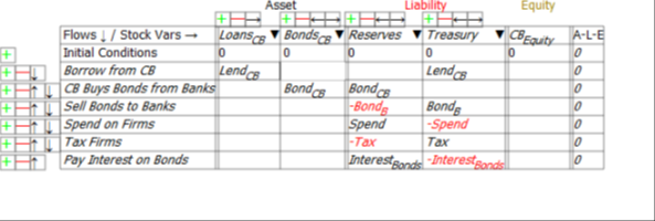
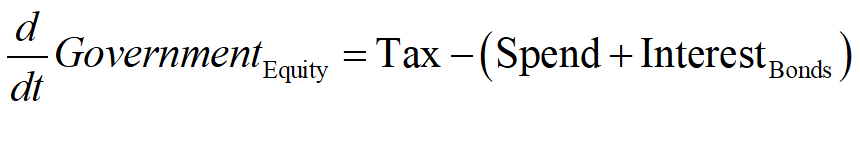
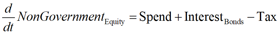
The danger to which Hern alludes is immediately apparent when we look at the Treasury’s Equity—the final column in Figure 2: if Treasury spending plus interest payments on outstanding Treasury Bonds exceeds taxation revenue, then its Equity will fall.
Figure 2: The Treasury’s accounts
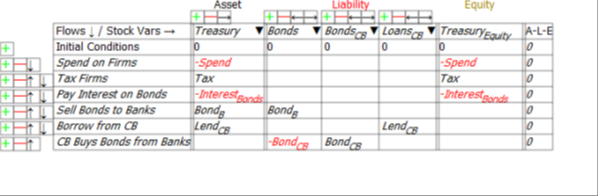
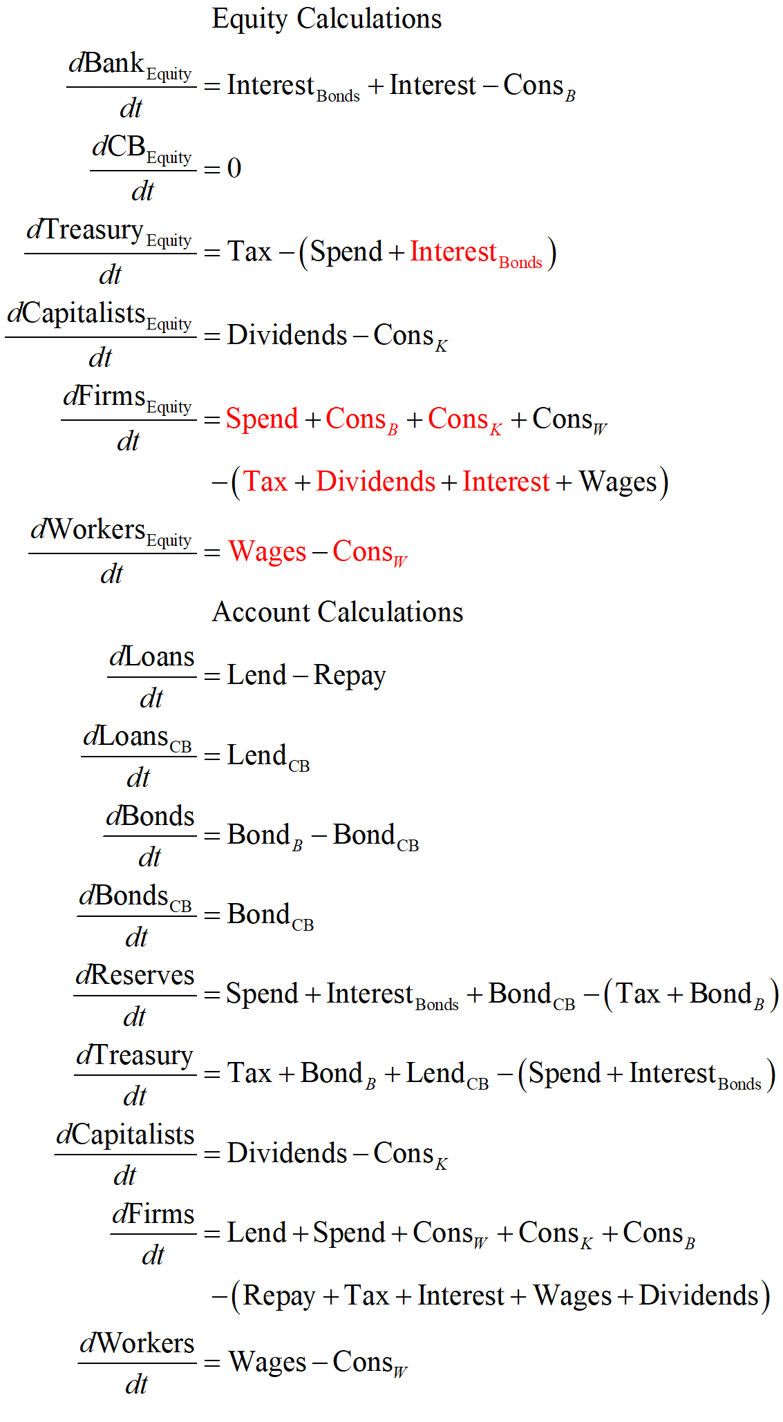
Mathematically, the rate of change of Treasury Equity is the sum of the flows Tax minus Spending minus Interest payments on Bonds held by the Banking Sector:
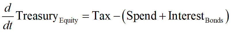
Given the initial conditions used in this post, in which Treasury Equity starts as zero, a deficit will immediately put the Treasury into negative equity.
This is not offset by the Central Bank, which comes out with no impacts on its equity position at all (note, this is not what I expected when I started building this model).
Figure 3: The Central Bank’s accounts
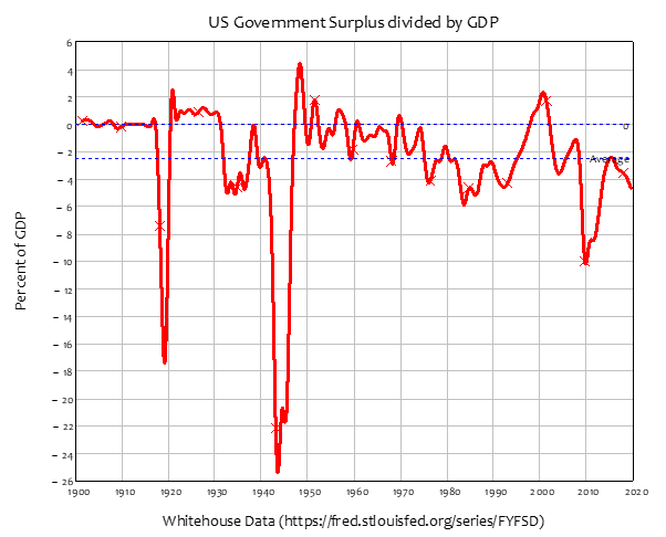
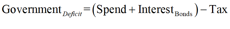
The rate of change of the Government’s Equity is therefore equal to its surplus—or the negative of its deficit, since the government has normally been in deficit for as long as records have been kept—see Figure 4. The only periods in which the Government has been in surplus for a sustained period are:
- The 1920s, between mid-1920 and mid-1931, a period of 11 years;
- The immediate post-WWII period, between early 1947 and mid-1949, a period of 2 years; and
- The late 1990s till early 2000s, between 1998 and early 2002, a period of 4 years.
Figure 4: US Government Surplus Divided by GDP. The average value is minus 2.48% of GDP
Returning to the model in this post, the impact of the Government deficit on the Government itself is entirely borne by the Treasury:
Summing the Treasury and Central Bank Equity equations to show the dynamics of the Government’s equity yields Equation :
Looked at just from the point of view of the Government sector then, running deficits is clearly “unsustainable, irresponsible, and dangerous”. If the government wants to have positive equity, then it should run a surplus. It’s an open and shut case—or so it appears, when looking just at the government’s books.
But in this model (and the real economy itself), one entity’s Asset is another’s Liability. So, to know whether a government surplus is a good idea for the system as a whole, we have to ask what the impact is of a government surplus on the rest of the economy?
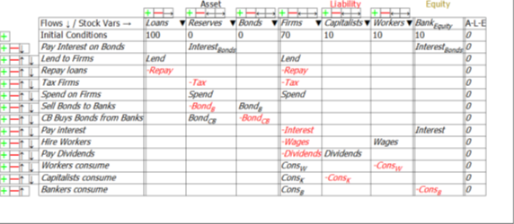
The rest of the economy is the NonGovernment Sector, the sum of the Banking Sector, and the “Non-Bank Private Sector“: the three non-Government and non-Bank sectors, Firms, Capitalists, and Workers. This model has been set up so that Capitalists and Workers are not directly affected by government spending and taxation, or interest payments on bonds, so we can answer this question just by looking at the economy from the Banking Sector’s point of view (Figure 5) and the Firm Sector’s point of view (Figure 6). The government actions that affect the equity of the Banking Sector and the Firm sector are shown at the top of each table.
The first line in Figure 5 shows that what is a negative for the equity of the Government Sector—paying interest to banks for their holdings of Treasury Bonds—is a positive for the Banking Sector.
Figure 5: The Banking Sector’s accounts
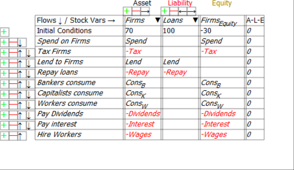
Similarly, first two lines of Figure 6 show that what is a negative for the equity of the Government sector is a positive for the Firm Sector, and that what is a positive for the Government is likewise a negative for the Firm Sector: Government spending increases the equity of the Firm Sector, and taxation reduces it.
Figure 6: The Firm Sector’s accounts
The non-Government net financial position is therefore the mirror image of the Government’s:
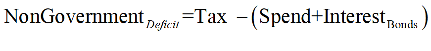
The deficit defines the flow, in dollars per year. Equity is the accumulation of that flow over time, in dollars. The NonGovernment sector’s equity is, like its deficit, the negative of the Government Sector’s Equity:
An integrated perspective on government finances thus reveals two undeniably uncomfortable truths:
- For the Government to run a surplus, the NonGovernment sector must run a deficit; and
- For the NonGovernment sector to be in positive equity, the Government Sector must be in identical negative equity.
Like two halves of a see-saw, both cannot be up at the same time. If the government runs a surplus—if the sum of interest payments on bonds plus spending is less than taxation—then the non-government sector is forced to run an identical deficit at that point in time. If the NonGovernment Sector is in positive equity, then the Government Sector must be in identical negative equity.
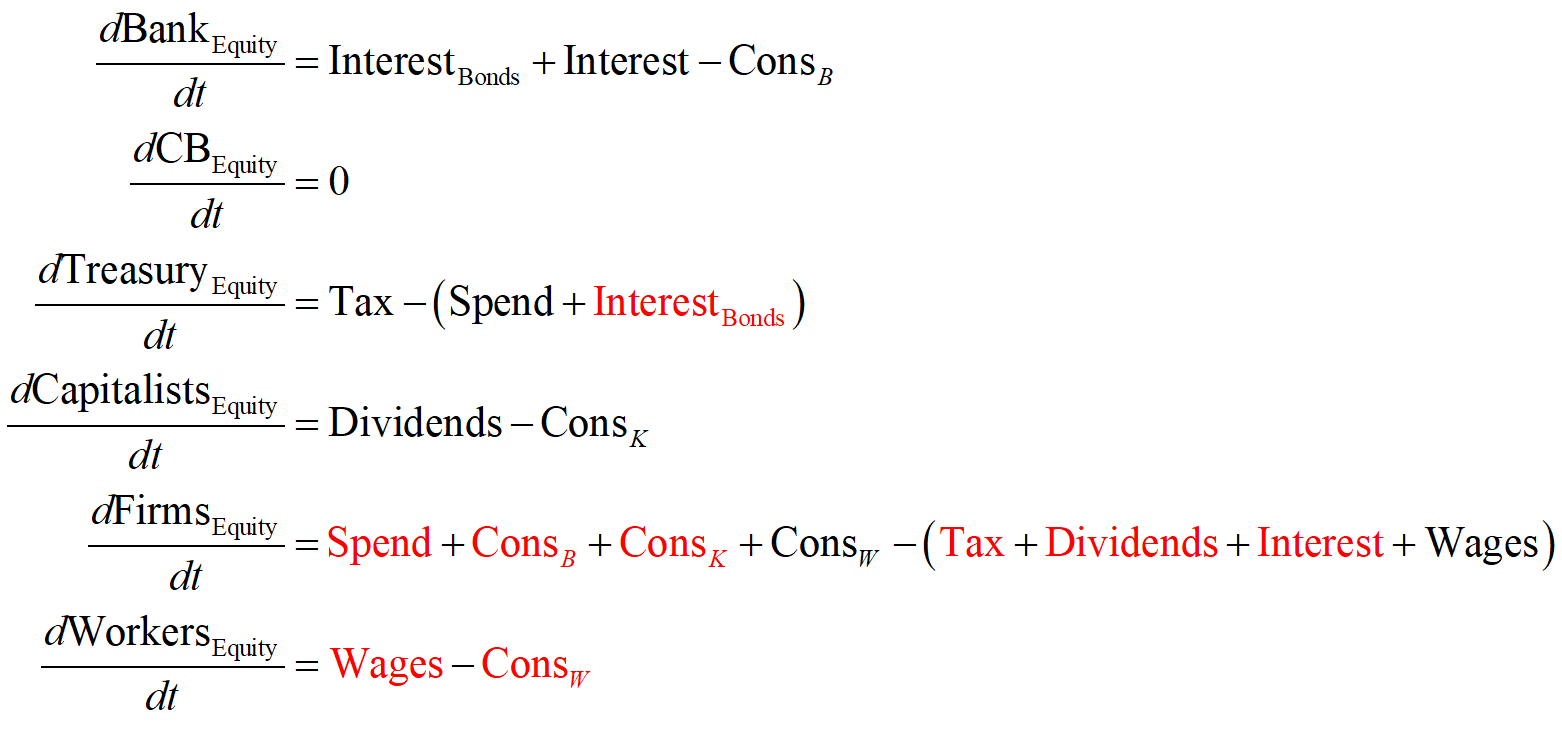
These outcomes are the macroeconomic consequences of the fact that one entity’s Asset is another’s Liability. The flows in Equations and show changes in Equity at one moment in time. Because these flows are identical in magnitude, but opposite in sign, at the aggregate level, the Equity of an entire economy is zero, and the rate of change of aggregate Equity is also zero.
Therefore, if one subset of the economy has positive equity, the remainder of the economy has identical negative equity. Equally, if the rate of change of one sector’s equity is positive, then the rate of change of the equity of the remainder of the economy is identical in magnitude, and negative. This is shown by Equation , where the first instance of a flow term is shown in black and the second instance in red: there are nine terms, each repeated twice, once as a positive and once as a negative. The sum is zero.
The question therefore is not whether deficits—and negative equity—are good or bad, but whose deficits and negative equity are sustainable or non-sustainable.
There is one sector that cannot be in persistent negative equity in a sustainable economic system: the Banking Sector. A bank must have positive Equity: it’s Assets must exceed the value of its Liabilities, otherwise it is bankrupt. Therefore, for a sustainable economic system, the Banking sector must necessarily be in positive Equity (periods when the Banking Sector as a whole is in negative equity are periods of extreme financial crisis, like 2007 and 1929).
It follows that the NonBank Sector—which is the sum of the Government plus, in this model, Firms, Capitalists and Workers—must be in negative equity. This is unavoidable, given that the sum of all Equity is zero. The only question is which subset of the non-Bank economy—the Government, or the NonBank Private Sector—will be in negative equity? Which sector is better placed to handle being in negative equity?
That question and others will be considered in a subsequent post.
Postscript
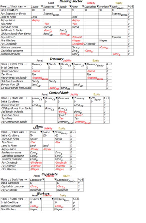
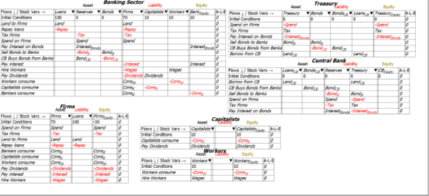
Figure 7 shows the full six Godley Tables that constitute this model, and Equation shows the differential equations generated by this model. If you’d like to explore this model yourself (it is attached to this post), download the latest beta release of Minsky from https://sourceforge.net/projects/minsky/files/beta%20builds/. The beta (currently version 2.19.0-beta.25) has features used here than are not in the current release version (Version 2.18). A subsequent post will define the flows used here to enable simulations, but the basic points of MMT are structural: they can be gleaned from the differential equations themselves, as I have done in this post.
Figure 7: Full Minsky MMT Model