This post collates three previous posts on modelling the domestic financial aspects of Modern Monetary Theory. There is a PDF of this post attached on my Patreon page, to aid offline reading. The Minsky model is also attached, and Minsky (which is free and Open Source) can be downloaded from https://sourceforge.net/projects/minsky/. This model uses features that are not in the current release version (version 2.18) so if you wish to run it, and 2.18 is still the release version, please download the latest beta version instead from https://sourceforge.net/projects/minsky/files/beta%20builds/.

I confess immediately that I chose the title because its acronym is a palindrome.

This model considers only the monetary aspects of MMT: the Job Guarantee and inflation management components are not yet incorporated. International trade and financial flows are not considered. However, the assertions of MMT about domestic monetary dynamics remain in dispute in economic and political circles, so it is worth putting these into a mathematical model where their veracity can be tested.

The primary stimulus for developing the model was the publication of Stephanie Kelton’s The Deficit Myth. Stephanie has written the book for non-technical readers, and she’s done a very good job: it’s a very easy read that explains why many conventional wisdoms about government spending are wrong. But MMT is facing heavy resistance in political and economic circles, with my favourite to date being a motion before the US Congress, posted by Representative Kevin Hern, to resolve:

That the House of Representatives (1) realizes that deficits are unsustainable, irresponsible, and dangerous; and (2) recognizes— (A) that the implementation of Modern Monetary Theory would lead to higher deficits and higher inflation; and (B) the duty of the House of Representatives to condemn Modern Monetary Theory.

The objective of this series of posts is to allow the assessment of the first part of this motion—the assertion that “deficits are unsustainable, irresponsible, and dangerous”.

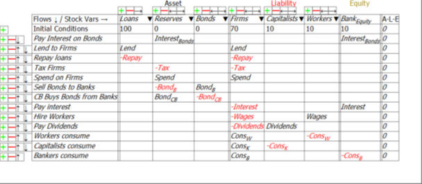
The models in this document are built in the Open Source system dynamics program Minsky, whose unique feature is the capacity to build models of financial flows using what are called Godley Tables (in honour of Wynne Godley, the pioneer of stock-flow-consistent-modelling). These tables enforce the “law of accounting” that (see Figure 1).

Figure 1: A blank Godley Table

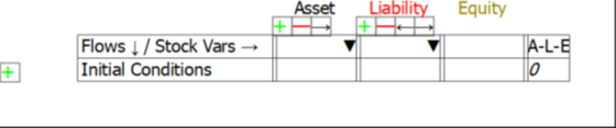
Once an account is flagged as an “Asset” for one entity, Minsky knows that it has to also be shown as a “Liability” for another entity. This
makes it possible to take an integrated look at the financial system, which allows us to assess Hern’s motion from the perspective of the entire monetary system, and not just the Government’s view of it.

An Integrated View of Deficits, Surpluses, and Equity

This Minsky model is a simple but complete model of a domestic monetary system. It has six sectors which can be divided into five components:

• The Treasury, and the Central Bank, which together constitute the Government Sector;
• The Banking Sector;
• The Firm Sector, Capitalists and Workers, which constitute the “NonBank Private Sector“;
• The NonBank Private Sector and the Banking Sector, which constitute the “NonGovernment Sector“; and
• The sum of the Government and the NonBank Private Sector, which constitute the “NonBank Sector“.

For simplicity, taxes—and government spending—are levied only on the Firm Sector, and banks make loans only to firms (the aggregate outcome would be the same if the model were generalized to have taxes and spending and loans in all sectors—it would just be much harder to read the tables).

There are just thirteen financial flows:

• Treasury spends on firms (Spend);
• Treasury taxes firms (Tax);
• Treasury sells bonds to the Banking Sector to cover any deficit (Bond_B);
• Treasury pays interest on Treasury Bonds owned by the Banking Sector (Interest_Bonds);
• The Central Bank buys and sells Treasury Bonds in “Open Market Operations” (Bond_CB);
• Banks lend to firms (Lend);
• Firms pay interest to Banks (Interest);
• Firms repay some debt to banks (Repay);
• Firms hire workers (Wages);
• Firms pay dividends (Dividends);
• Workers buy goods from firms (Cons_W);
• Capitalists buy goods from firms (Cons_K); and
• Bankers buy goods from firms (Cons_B).

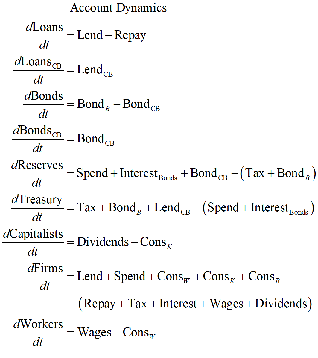
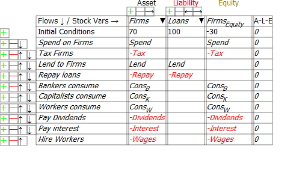
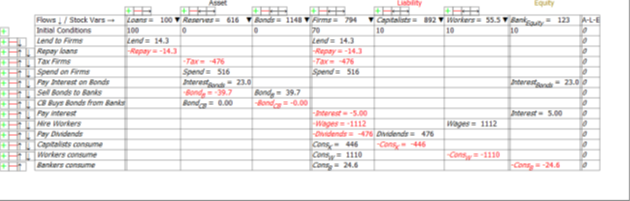
Minsky provides an integrated view of how these flows interact to determine the financial position of each of the six sectors in the model in interlocking double-entry bookkeeping tables. It generates differential equations from these flows that show how the stocks—the financial accounts—change over time.

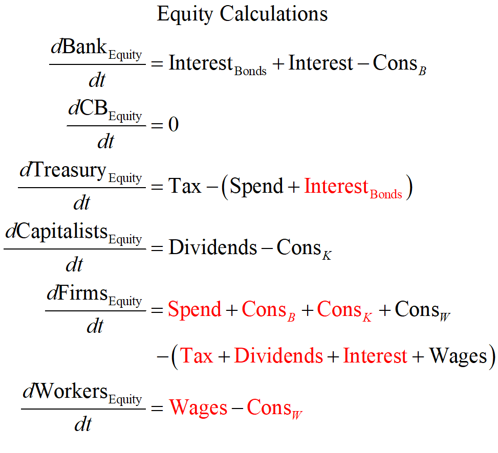
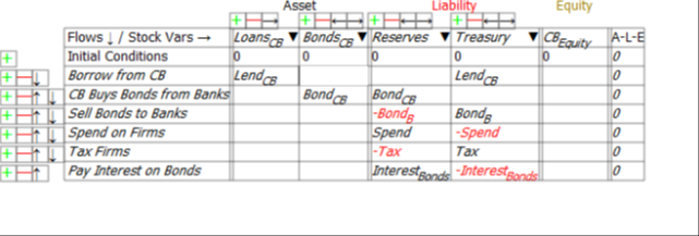
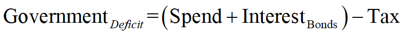
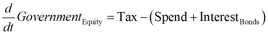
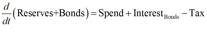
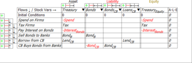
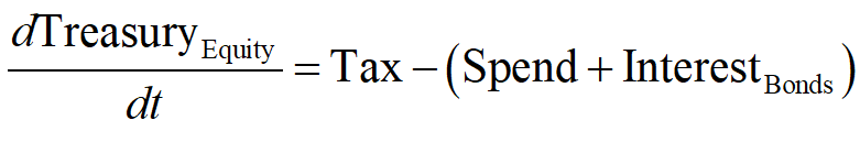
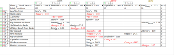
The danger to which Hern alludes is immediately apparent when we look at the Treasury’s Equity—the final column in Figure 2: if Treasury spending plus interest payments on outstanding Treasury Bonds exceeds taxation revenue, then its Equity will fall.

Figure 2: The Treasury’s accounts

Mathematically, the rate of change of Treasury Equity is the sum of the flows Tax minus Spending minus Interest payments on Bonds held by the Banking Sector:

         

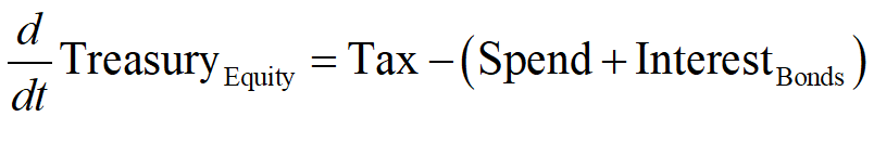
Given the initial conditions used in this post, in which Treasury Equity starts as zero, a deficit will immediately put the Treasury into negative equity.

This is not offset by the Central Bank, which comes out with no impacts on its equity position at all (note, this is not what I expected when I started building this model).

Figure 3: The Central Bank’s accounts

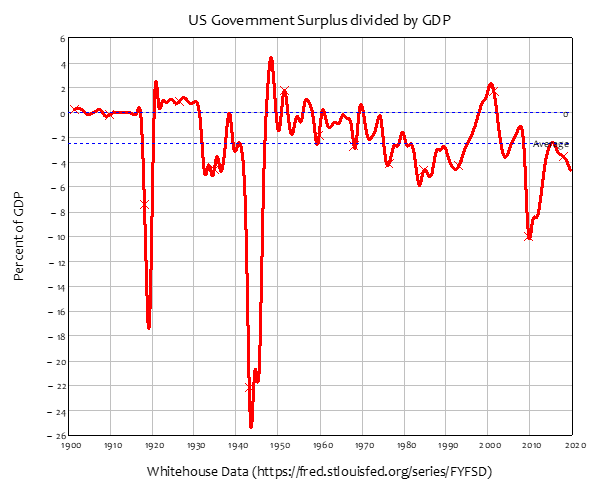
The rate of change of the Government’s Equity is therefore equal to its surplus—or the negative of its deficit, since the government has normally been in deficit for as long as records have been kept—see Figure 4. The only periods in which the Government has been in surplus for a sustained period are:

• The 1920s, between mid-1920 and mid-1931, a period of 11 years;
• The immediate post-WWII period, between early 1947 and mid-1949, a period of 2 years; and
• The late 1990s till early 2000s, between 1998 and early 2002, a period of 4 years.

Figure 4: US Government Surplus Divided by GDP. The average value is minus 2.48% of GDP

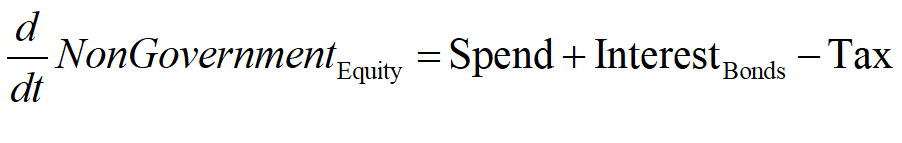
Returning to the model in this post, the impact of the Government deficit on the Government itself is entirely borne by the Treasury:

         

Summing the Treasury and Central Bank Equity equations to show the dynamics of the Government’s equity yields Equation :

         

Looked at just from the point of view of the Government sector then, running deficits is clearly “unsustainable, irresponsible, and dangerous”. If the government wants to have positive equity, then it should run a surplus. It’s an open and shut case—or so it appears, when looking just at the government’s books.

But in this model (and the real economy itself), one entity’s Asset is another’s Liability. So, to know whether a government surplus is a good idea for the system as a whole, we have to ask what the impact is of a government surplus on the rest of the economy?

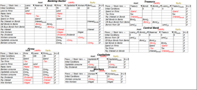
The rest of the economy is the NonGovernment Sector, the sum of the Banking Sector, and the “Non-Bank Private Sector“: the three non-Government and non-Bank sectors, Firms, Capitalists, and Workers. This model has been set up so that Capitalists and Workers are not directly affected by government spending and taxation, or interest payments on bonds, so we can answer this question just by looking at the economy from the Banking Sector’s point of view (Figure 5) and the Firm Sector’s point of view (Figure 6). The government actions that affect the equity of the Banking Sector and the Firm sector are shown at the top of each table.

The first line in Figure 5 shows that what is a negative for the equity of the Government Sector—paying interest to banks for their holdings of Treasury Bonds—is a positive for the Banking Sector.

Figure 5: The Banking Sector’s accounts

Similarly, first two lines of Figure 6 show that what is a negative for the equity of the Government sector is a positive for the Firm Sector, and that what is a positive for the Government is likewise a negative for the Firm Sector: Government spending increases the equity of the Firm Sector, and taxation reduces it.

Figure 6: The Firm Sector’s accounts

The non-Government net financial position is therefore the mirror image of the Government’s:

         

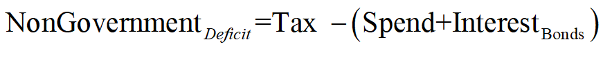
The deficit defines the flow, in dollars per year. Equity is the accumulation of that flow over time, in dollars. The NonGovernment sector’s equity is, like its deficit, the negative of the Government Sector’s Equity:

         

An integrated perspective on government finances thus reveals two undeniably uncomfortable truths:

• For the Government to run a surplus, the NonGovernment sector must run a deficit; and
• For the NonGovernment sector to be in positive equity, the Government Sector must be in identical negative equity.

Like two halves of a see-saw, both cannot be up at the same time. If the government runs a surplus—if the sum of interest payments on bonds plus spending is less than taxation—then the non-government sector is forced to run an identical deficit at that point in time. If the NonGovernment Sector is in positive equity, then the Government Sector must be in identical negative equity.

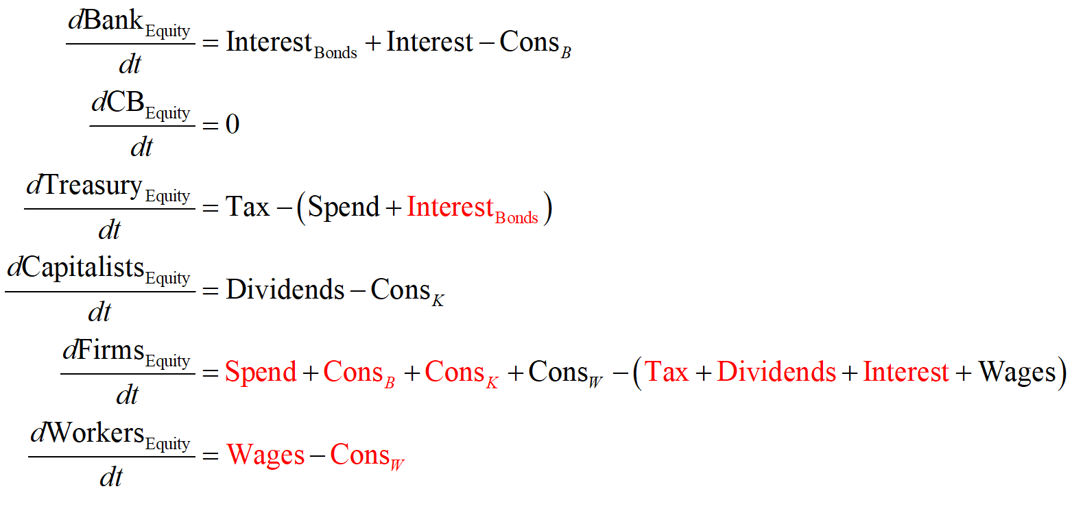
These outcomes are the macroeconomic consequences of the fact that one entity’s Asset is another’s Liability. The flows in Equations and show changes in Equity at one moment in time. Because these flows are identical in magnitude, but opposite in sign, at the aggregate level, the Equity of an entire economy is zero, and the rate of change of aggregate Equity is also zero.

Therefore, if one subset of the economy has positive equity, the remainder of the economy has identical negative equity. Equally, if the rate of change of one sector’s equity is positive, then the rate of change of the equity of the remainder of the economy is identical in magnitude, and negative. This is shown by Equation , where the first instance of a flow term is shown in black and the second instance in red: there are nine terms, each repeated twice, once as a positive and once as a negative. The sum is zero.

         

The question therefore is not whether deficits—and negative equity—are good or bad, but whose deficits and negative equity are sustainable or non-sustainable.

There is one sector that cannot be in persistent negative equity in a sustainable economic system: the Banking Sector. A bank must have positive Equity: it’s Assets must exceed the value of its Liabilities, otherwise it is bankrupt. Therefore, for a sustainable economic system, the Banking sector must necessarily be in positive Equity (periods when the Banking Sector as a whole is in negative equity are periods of extreme financial crisis, like 2007 and 1929).

It follows that the NonBank Sector—which is the sum of the Government plus, in this model, Firms, Capitalists and Workers—must be in negative equity. This is unavoidable, given that the sum of all Equity is zero. The only question is which subset of the non-Bank economy—the Government, or the NonBank Private Sector—will be in negative equity? Which sector is better placed to handle being in negative equity?

 

That question and others are considered in the next section.

The dynamics of money

The previous section finished with the observation that, since the sum of all Equity is zero, and the banking sector must be in positive equity, part of the remainder of the economy—the government, or the non-bank public—must be in negative equity. So which sector is better equipped to handle that: the non-bank public, or the government?

This will raise the age-old question that is perennially thrown at those who advocate government spending: “How are you going to pay for it?”, or “Where’s the money going to come from?”. To answer both these questions, we first need to know how money is created in general.

Since money, exclusively in this model and primarily in the real world, is the sum of the Banking Sector’s Liabilities and Equity, any action which increases Bank Liabilities and Equity creates money. Since every transaction is recorded twice, operations which increase the money supply must therefore occur on both the Assets and the Liabilities/Equity sides of the banking sector’s ledger. Operations which occur exclusively on either the Assets side, or the Liabilities/Equity side, shift money between accounts and do not create money.

So the answer to the “where’s the money going to come from?” question is “from any operation which increases the Assets and Liabilities/Equity of the banking sector”. Equally, any operation that reduces Assets and Liabilities/Equity destroys money.

Only 5 of the 13 flows in this model affect both the Asset and Liabilities/Equity sides of the banking sector’s ledger: Lending (and Repayment); Government spending (and Taxation); and interest payments on Treasury Bonds. These are shown in the top 5 rows of Figure 7. All other operations are either Liability/Equity swaps, or Asset swaps, and they don’t create money.

Figure 7: The Banking Sector’s Ledger

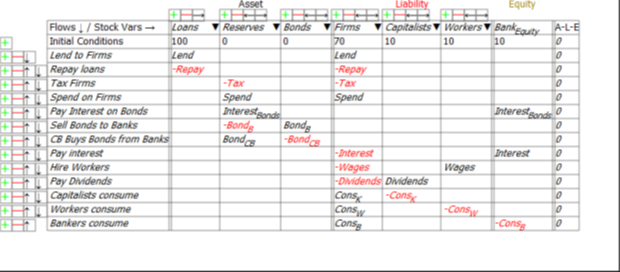
Operations that don’t create money include the usual suspects—payment of interest on loans by firms (which transfers money from the Firm Sector to the Banking Sector), purchases of goods from the Firm Sector by workers, capitalists and bankers. But they also include two operations that figure large in conventional arguments about how to pay for government spending: sales of Treasury Bonds to the finance sector; and purchases of Treasury Bonds from the finance sector by the Central Bank in “Open Market Operations” (which are primarily used to control the rate of interest). Neither of these operations create money.

They are asset swaps: the sale of Treasury Bonds to the finance sector (the “Banking Sector” in this model) reduces Reserves and increases the Banking Sector’s stock of Treasury Bonds. The purchase of Treasury Bonds from the Banking Sector by the Central Bank reduces the Banking Sector’s stock of Treasury Bonds and increases the Banking Sector’s Reserves. Neither operation affects the amount of money in the economy—the sum of the Liabilities plus Equity of the Banking Sector.

Since it’s an asset swap for the Banking sector to buy Treasury Bonds using Reserves, the answer to “where’s the money going to come from?” is “from operations that increase the sum of Reserves and Bonds”. You can work this out by adding up the entries in the Reserves and Bonds columns of Figure 7: the Banking sector assets Reserves plus Bonds will grow if government spending plus interest payments on Treasury Bonds exceed taxation:

         

The Reserves that are used to buy the Bonds thus come from the deficit itself. The deficit—the extent to which government spending and interest payments exceeds taxation—creates money in private sector bank accounts (the Firm Sector and Bank Equity only in this model). This boosts the Liabilities and Equity of the Banking Sector. The corresponding Asset that is increased by the deficit is the Reserve accounts of the banking sector. If no interest is paid on Reserves—the “usual” situation, and sometimes made worse by charging negative interest on Reserves in the false belief that this will encourage Banks to lend more—then the Banks have a positive incentive to use these reserves to buy Treasury Bonds instead.

So the answer to the “Where’s the money going to come from?” to pay for the deficit question is that it comes from the deficit itself: the deficit creates money that can be spent in the private sector; and it creates Reserves, which are (usually) non-interest earning Assets of the Banking Sector that are liabilities of the Central Bank—see Figure 8.

Figure 8: The Central Bank’s Ledger

Reserves are Assets of the Banking Sector that earn it no income. But if the Treasury issues bonds to cover the deficit—if the total value of Treasury Bonds offered for sale is equal to the deficit itself—then the Banking Sector is offered a deal to swap a non-income-earning asset for an income-earning one.

What do you think the banks would do, when offered that deal? They take it, of course: this is why Treasury Bond Auctions have always been over-subscribed. Selling the bonds themselves is not a problem. It is, as Kelton emphasises in The Deficit Myth, a “no brainer” swap of a zero-income-asset for a positive-income-asset.

The money needed to buy the bonds has already been created, and is sitting in the Reserve account. Banks then transfer their funds from one Asset that earns no income (Reserves) to another Asset that does (Treasury Bonds). This Asset is a liability, not of the Central Bank, but of the Treasury itself—see Figure 9.

Figure 9: The Treasury’s Ledger

This table also shows that the increase in Reserves is caused by the fall in the Government’s equity: Reserves (and hence money) rise if the Government runs a deficit; Reserves and money fall if the Government runs a surplus:

         

How does the Treasury pay the interest on the bonds? The same way it pays for spending in excess of taxation: it runs up its own negative equity—see the final column in Figure 9.

This can be done in two ways, as indeed can overall deficit-financing itself: by the Treasury having a negative balance in its account at the Central Bank; or if the Treasury borrows from the Central Bank to pay Interest on the Bonds (the second last row of Figure 9). If it does so, the negative equity from paying interest on the bonds remains, but the Treasury Account at the Central Bank can be kept non-negative.

A third option is that the Central Bank buys the bonds off the Banking Sector in Open Market Operations (or QE). If it does so, the amount of interest the Treasury needs to pay falls. Also, since the Treasury is the effective owner of the Central Bank, it doesn’t need to pay interest to the Central Bank on its holdings of Treasury Bonds—or if it does, the interest payments come back to the Treasury in Central Bank profits.

So the Government can run a deficit, and pay interest on the Treasury Bonds issued to cover it (not finance it: the deficit is self-financing in that it creates money), so long as it is willing to countenance being in negative equity. As noted in the previous post, because Banks must be in positive equity, the non-Banking sectors (and that includes the Government) must be in negative equity. For the Government to achieve positive equity therefore—which seems desirable, if you take the partial view of the economy epitomised by Representative Hern’s motion that “deficits are unsustainable, irresponsible, and dangerous”—the non-Bank private sector must be pushed into even greater negative equity.

Does that sound like a good idea?

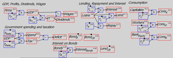
To show the consequences for the economy of the government running a deficit or a surplus, it’s necessary to go beyond the purely structural equations used so far, and to consider some simulations. In what follows, I’ve built an extremely simple model of monetary dynamics in which all expenditures depend on the amounts of money in relevant bank accounts. There are many other ways these expenditures could be modelled, but this way ensures fairly easily that crazy outcomes—like workers have negative bank balances, but still spending their wages—don’t happen in this very simple model.

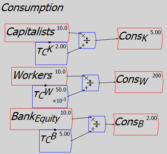
For example, I relate consumption by workers to the level of workers deposit accounts at the private banks, using the engineering concept of a “time constant”. This is a number that tells you how long an action would take to run an account down to zero, if it’s removing money from the account, or to double it, if it’s adding money to an account. A time constant of 0.02 for workers consumption says that if workers consumed at a constant rate, and there were no other inflows or outflows in their accounts, then they would run their accounts down to zero in 1/50^th of a year—roughly a week. Higher values for capitalists and bankers—say 2 for capitalists and 5 for bankers—assert that it would take 2 years and 5 years respectively for them to run their accounts down to zero through consumption alone.

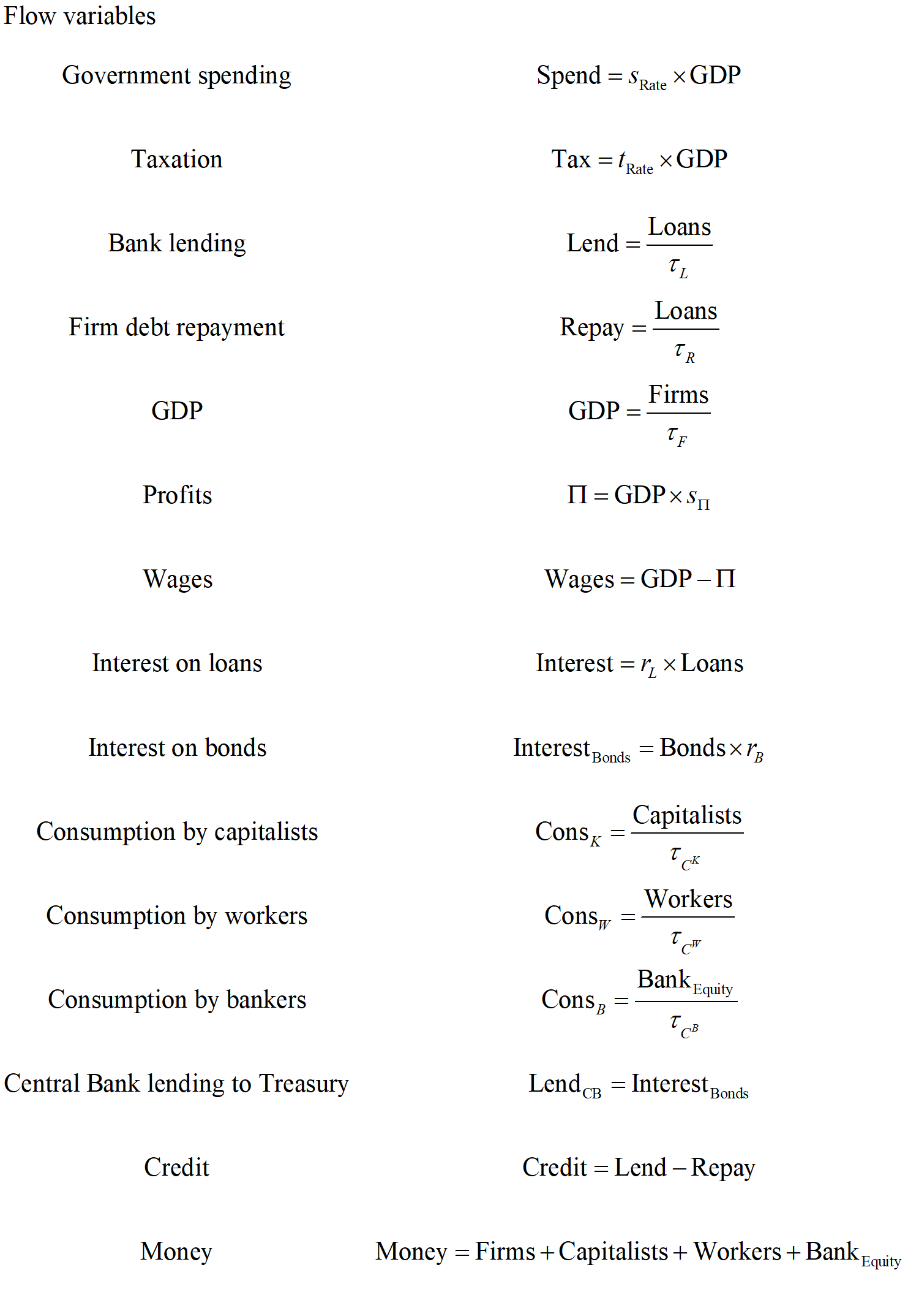
You divide the relevant stock (the level of bank accounts, in the case of consumption) by the time constant to get the annual flow—see Figure 10.

Figure 10: Equations for consumption

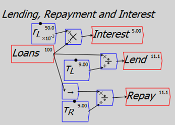
Similarly, a time constant of 9 for bank lending says that if this was the only inflow affecting the level of debt, and it went on at a constant rate, debt would double in 9 years. Repayment with the same time constant means that the level of (private) debt remains constant.

Figure 11: Modelling interest payments, lending and repayment

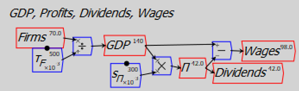
GDP is treated as the turnover of money in the firm sector (it can also be treated as the sums of consumption and investment—which investment is entirely debt-financed in this model—and net government spending, but that makes it possible to end up with negative sums in deposit accounts, unless a much more complicated model is constructed).

Figure 12: Modelling GDP and income distribution

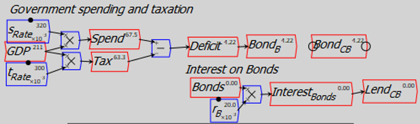
Government spending and taxation are treated as simple percentages of GDP. For the moment, I have not considered how they are financed, so the flows Bonds_B, Bonds_CB and Interest_Bonds are not wired up. The equations that define the system’s flows at this point are shown in Figure 13. At this stage, sales of Treasury Bonds to the Banking Sector, Central Bank purchases of Bonds from the Banks, and Treasury borrowing from the Central Bank, are not defined.

Figure 13: All the flow equations in the model (without bond sales or interest on bonds)

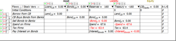
With no explicit financing of a government deficit, the negative equity that this causes for the government turns up as a negative balance in the Treasury’s account at the Central Bank—see Figure 14, which shows the impact of a 2% of GDP deficit for 60 years on the Treasury. It runs accumulates negative equity of $160, and that is entirely due to its account at the Central Bank being negative to the tune of $160.

Figure 14: The Treasury’s Ledger with no bond sales: negative Treasury Account and Treasury Equity

Figure 15 shows the impact of a 2% of GDP deficit for 60 years from the Central Bank’s perspective, and the key point is that the negative equity of the Treasury is the same magnitude as the positive Reserves of the Banking Sector: the accumulated deficits of the Government are precisely equal to the accumulated Reserves of the Banking Sector.

Figure 15: The Central Bank’s Ledger with no Bond sales: negative Treasury precisely equals positive Reserves

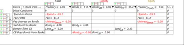
How does the picture change if we require that the Treasury’s account at the Central Bank can’t go into overdraft? Then the Treasury has to sell Bonds equal to its Deficit, and borrow from the Central Bank to pay interest on those bonds.

Figure 16: Bond sales are equal to the deficit, no Central Bank purchases of Bonds from the Banking Sector

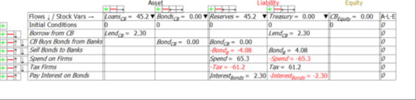
Running this model to the same point as the previous one, where the Treasury Equity reaches minus $160, this negative equity consists of $115 in Bonds and $45.2 in Loans from the Central Bank (see Figure 17; the Treasury account at the Central Bank remains at zero). The Bond sales represent the accumulated government deficit over time, while the Loans from the Central Bank represent the accumulated interest on those bonds.

Figure 17: Treasury books with Bond sales covering the deficit

Can the Central Bank afford to lend the money to pay the interest on Treasury Bonds to the Treasury? Yes: as Figure 18 shows, the loans to the Treasury are an Asset of the Central Bank. It has the capacity to expand its balance sheet indefinitely, and none of the operations shown in this model affect its equity at all.

Figure 18: Central Bank books with Bond sales and interest payments on Bonds

I have to note that this was a surprise to me: I had guessed that the government’s negative equity would be carried by the Central Bank, and the fact that a Central Bank—unlike a private one—can operate with negative equity (David Bholat and Robin Darbyshire, 2016) would be what enabled the government as a whole to sustain negative equity. But it turned out that my guess was wrong: the Central Bank simply acts as an enabler of and conduit for the Treasury’s negative equity.

Does the fact that the Treasury is borrowing from the Central Bank (in this model) cause any difficulty? No, because while private individuals can’t pay interest on loans by borrowing from banks—without that interest ballooning with further interest and driving us bankrupt—the Treasury can pay interest on Bonds to the Banking Sector by borrowing from the Central Bank because, technically and legally, the Treasury owns the Central Bank. It therefore doesn’t have to pay interest on any loans from the Central Bank If it did, it would get that money back in dividend payments from the Central Bank anyway.

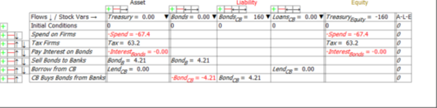
What happens if the Central Bank buys all the Bonds from the Banks? Then the negative equity of the Treasury consists entirely of its debt to the Central Bank (see Figure 19).

Figure 19: Treasury’s books with Central Bank Open Market Operations purchasing all Treasury Bonds

Since those Bonds have been purchased off the Banking Sector, the Banking Sector has Reserves of 160 (see Figure 20). This is not as desirable a situation for the Banks as when they own the bonds, because with no Treasury Bonds they receive no interest payments from the Government. Far from the finance sector in general having “Bond Vigilantes” ready to deny the government bond sales if they’re worried about the state of government finances, the “Bond Vigilantes” are vigilantly on the lookout for sales of Treasury Bonds so that they can swap out of a non-income-earning asset and into an income-earning one.

Figure 20: Banking Sector’s books with OMOs buying 100% of Bonds

In the next section, I consider what the impact is of different fiscal regimes: the government running a deficit (as the USA has for most of the last 120 years—roughly of 2.5% of GDP); the government running a surplus; the government running a surplus and the private sector borrowing from the Banking Sector; the government running a surplus and the private sector reducing its debt to the Banking Sector; and the government running a deficit while the private sector increases its debt to the Banking Sector.

Simulating monetary dynamics

The previous section confirmed the MMT assertion the deficit creates the funds (in Bank Reserves) that are used by the finance sector to buy Treasury Bonds. Therefore, leaving aside the foreign sector and countries like those in the EU that don’t issue their own currency, there is never a problem with a government selling bonds to cover a deficit: their purchase is actually a favourable asset swap for the finance sector, exchanging non-income-earning Reserves for income-earning Bonds.

Though this is still a very simple and stylized model, it lets us do something we can’t do in the real world: separate out the economic impact of the government undertaking a policy from the private sector’s reaction to that policy. This allows us to isolate causal factors when there is more than one cause at play. That’s vitally necessary to be able to interpret historical data on whether running deficits is a good idea or not, because (leaving aside the foreign sector) there are two ways to create money: by the government running a deficit, or by the banks lending out more than they get back in repayments.

Historical Deficits & Surpluses

The US government has, on average over the last 120 years, run a deficit equivalent to 2.3% of GDP. The post-WWII average has been -2.5%—see Figure 21. The peak deficit occurred during WWII, at almost 26% of GDP.

Figure 21: US Government surplus since 1900

These deficits, and some surpluses—most notably, the decade of the 1920s, and the late Clinton to early Bush II years—have led to the Government debt to GDP ratio varying substantially over time—see Figure 22.

Figure 22: The US Government’s debt to GDP ratio since 1790

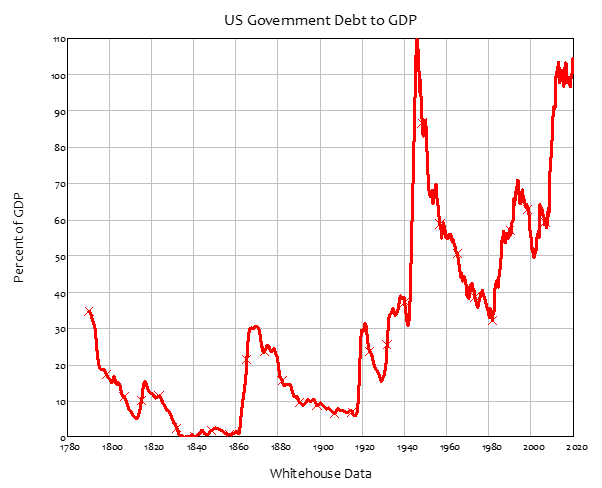
The relationship between deficits and the government debt to GDP ratio is not straightforward: there are substantial periods where the government is running a deficit and the debt ratio is falling. The clearest example of this is between 1950 and 1980, when there were only brief periods of surplus and the deficit averaged 1% of GDP; the government debt ratio fell from 87% of GDP to 34% of GDP over that time. This period includes the so-called “Golden Age of Capitalism” between the start of the 1950s and the middle of the 1970s, when GDP growth was high, and unemployment and inflation were low.

 

Figure 23: Government Debt Ratio vs Government Surplus

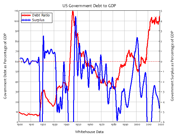
But there were also “Gilded Ages”—like the 1920s and the Clinton Years till 9/11—when the government ran a surplus and the economy boomed. During these periods, surpluses were lauded as a sign of true economic success.

This was President Calvin Coolidge’s position. He maintained a 1% of GDP surplus throughout his term, and in his final State of the Union speech in December 1928, he lauded his surplus as the cause of the prosperity of the 1920s:

No Congress of the United States ever assembled, on surveying the state of the Union, has met with a more pleasing prospect than that which appears at the present time…

We have substituted for the vicious circle of increasing expenditures, increasing tax rates, and diminishing profits the charmed circle of diminishing expenditures, diminishing tax rates, and increasing profits.

Four times we have made a drastic revision of our internal revenue system, abolishing many taxes and substantially reducing almost all others. Each time the resulting stimulation to business has so increased taxable incomes and profits that a surplus has been produced. One-third of the national debt has been paid, while much of the other two-thirds has been refunded at lower rates, and these savings of interest and constant economies have enabled us to repeat the satisfying process of more tax reductions. Under this sound and healthful encouragement the national income has increased nearly 50 per cent, until it is estimated to stand well over $90,000,000,000. It has been a method which has performed the seeming miracle of leaving a much greater percentage of earnings in the hands of the taxpayers with scarcely any diminution of the Government revenue. That is constructive economy in the highest degree. It is the corner stone of prosperity. It should not fail to be continued. {Coolidge, 1928 #6057}

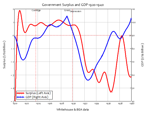
Looking at the data, it appears that Coolidge had a point: GDP rose from $70 billion to over $100 billion across the 1920s, as his government maintained a surplus of about $1 billion per year. Did the surplus cause the “Roaring Twenties” boom? In a classic case of “correlation is not causation”, superficially it seems that the decline into a deficit caused the Great Depression.

Figure 24: Government surplus and GDP 1920-1940

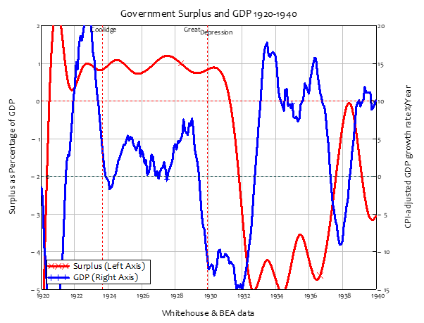
However, the decline in the growth rate, from 7% to minus 10%, preceded the change from surplus to deficit (see Figure 25), so perhaps the Great Depression caused the change from surplus to deficit. Also, after the original crash between 1920 and 1932, the rate of real economic growth was extremely high between 1933 and 1936, exceeding 10% per annum when the deficit was 5% of GDP. A return to a balanced budget (if not quite a surplus) between 1937 and 1938 coincided with a collapse in economic growth, from over 15% per annum in 1936 to almost minus 10% in 1938.

Figure 25: Surplus as % of GDP versus real GDP growth rate

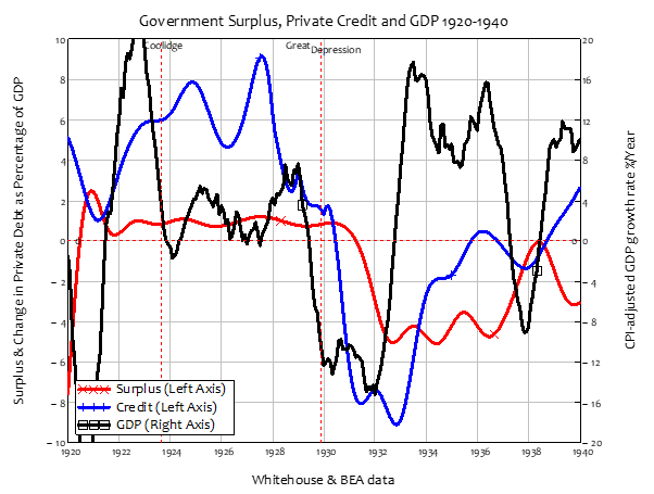
This analysis ignores the factor that (following Irving Fisher and Hyman Minsky) I focus upon as the main cause of capitalism’s booms and busts: private credit. As Figure 26 shows, credit was positive during the 1920s, and negative during the 1930s—matching much more closely the pattern of GDP change. It was also much bigger than the government surplus or deficit: credit was as high as 9% of GDP in 1929, versus a surplus of 1%; and it was as low as -9% of GDP in 1933, versus a deficit of 5%.

Figure 26: Surplus, Credit, and Change in GDP

Let’s cut through this historical confusion with some simple simulations using this model in which we can separate out periods of deficit and surplus from periods of private sector leveraging and deleveraging.

Phase 1: A deficit for 100 years

The first simulation has a deficit of 2.5% of GDP—roughly equal to the average US government deficit since 1900—for 100 years. Spending is 32.5% of GDP and taxation is 30% of GDP. The Treasury sells Treasury Bonds to the Banks, and pays interest on those bonds to the Banks by borrowing from the Central Bank.

Figure 27: Deficit for 100 Years

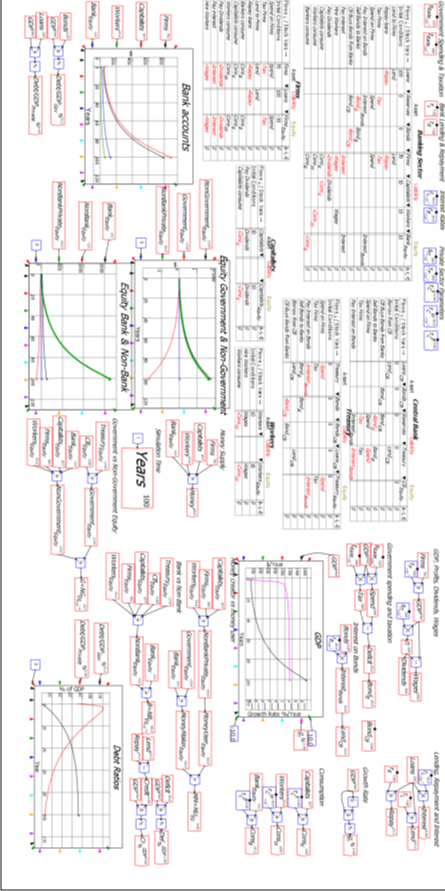
The deficit is expansionary, and pushes the whole private sector—Firms, Capitalists and Workers as well as Banks—into positive equity, to the tune of $1,734. This positive equity is of course precisely equal in magnitude to the negative equity of the Treasury of $1,734.

At the end of this part of the simulation, the total assets of the banking sector are $1,834, backing an identical amount of money in the bank accounts of the non-bank private sector plus the banking sector’s equity. This is split between $100 in private debt (of the Firm sector), $616 in Reserves created entirely by the interest being paid on Bonds, and $1,148 in Bonds, created entirely by the government deficits.

Because there is no private sector borrowing, the private sector debt ratio also falls, from 70% of GDP at the beginning of the simulation to 6.3% by the end, as GDP rises from $140 per year to $1,588 at the end. Because the Treasury is selling Treasury Bonds to match the deficit and maintain its account at the Central Bank at a $0 balance, the ratio to GDP of Treasury Bonds owned by the Banking Sector rises from zero to 72% of GDP—at which point the “deficit hawks” are likely to intervene and insist that the government “gets its books in order” by running a surplus.

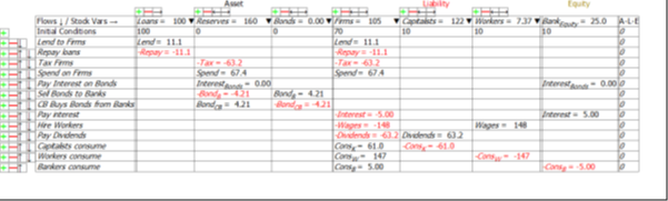
Figure 28: Banking sector’s books after 100 years of a 2.5% of GDP Deficit

 

Phase 2: A 1% of GDP surplus until Government Debt hits 10% of GDP

In this next phase, the government runs a 1% of GDP surplus by reducing spending to 29% of GDP. The immediate effect of this surplus is a slowdown in the rate of growth of GDP, from 4% p.a. to initially -2%. The growth rate bounces back for a while, but ultimately turns negative, and by the time the Government debt ratio has hit the 10% of GDP target (after 64 years), GDP has fallen from $1,588 per year to $1,418 per year.

Figure 29: A 1% of GDP surplus until government debr ratio hits 10%

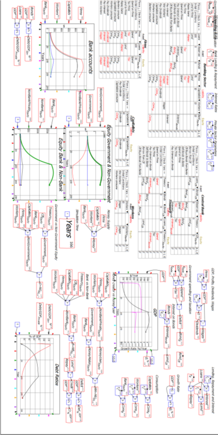
The government’s debt level—the ratio to GDP of Treasury Bonds owned by the Banking sector—has fallen from 72% of GDP ($1,148/$1,1588) to 10% ($144/$1,430), as intended. However, the scale of the government’s negative equity has barely shifted, from $1,734 to $1,581. The reason is that a substantial part of the money that was created in Phase 1 was via interest payments on Bonds, which were financed by borrowing from the Central Bank. Even though Bonds owned by the Banks were declining at the rate of 1% of GDP per year, the interest on the outstanding debt remained high initially. These interest payments created money, countering the destruction of money by the surplus. The momentum of this plunged towards the end, hence the rate of decline of GDP increased.

The same effect applies with private sector equity, which reaches a peak when the additions to private sector equity from interest on Treasury Bonds is matched by the cancellation of bonds by the surplus. Then it falls as the scale of the government’s negative equity also falls. A surplus thus depresses economic activity, and reduces private sector equity.

But that’s not what Calvin Coolidge saw, and claimed: he claimed that a surplus causes the economy to boom, not slump. What was he, and this simulation, missing?

Phase 3: A surplus and Private sector borrowing

It, and Calvin Coolidge, missed the private sector borrowing. This simulation starts from the same point as Phase 2, but as well as the government running a 1% of GDP surplus, there is also net private sector borrowing as the time constant on lending falls to 5 years and that for repayment rises to 9 years. Credit is as high as 11% of GDP.

 

Figure 30: A surplus and private sector borrowing

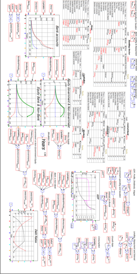
Here the economic performance appears much better: GDP growth is sustained, and by the time the government debt ratio hits the target of 10% of GDP—after a mere 38 years in this simulation versus 64 year in the surplus-only case—GDP has risen from $1,588 per year to $3,529—a total boom.

However, because this was a boom financed by the firm sector borrowing money from the banks, by the end of it, the private debt to GDP ratio has risen from 6% to 79% of GDP. This is a bigger rise in private debt that occurred during the 1920s—and then abruptly went into reverse in 1920 (see Figure 31).

Figure 31: Private sector debt and credit (change in private debt per year) 1920-1940

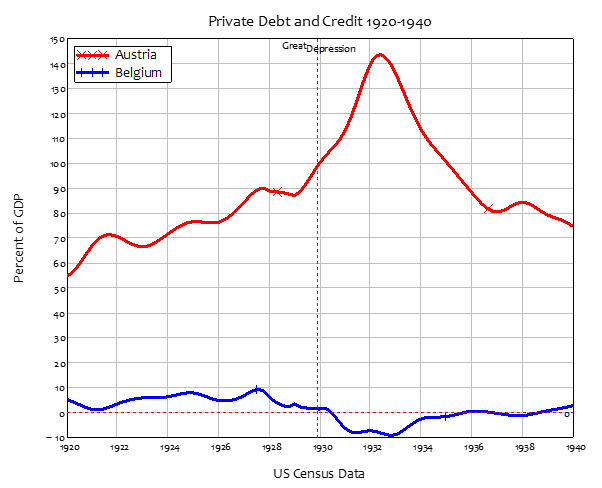
Figure 32: The Banking sector’s books after 38 years of a 1% of GDP surplus and private sector borrowing.

What happens to the economy in this model if the private sector switches from borrowing to deleveraging while the government is still running a surplus?

Phase 4: Government surplus and private sector deleveraging

The answer, in so many words, is a Depression. With both the government surplus and private sector deleveraging taking money out of the economy, GDP plunges, from $3,529 when deleveraging began to $1614 just 12 years later.

Figure 33: The private sector switches from borrowing to deleveraging

What happens if, as occurred during the 1930s, the government switches from a 1% of GDP surplus to a 5% of GDP deficit, while the private sector continues to de-lever?

The result is a return to growth, as the deficit counteracts the reduction in the money supply caused by private sector deleveraging.

Figure 34: Government switches from Coolidge surplus to Roosevelt Deficit

Phase 0: What should be done?

I hope the previous simulations have clarified that some deficits are indeed “unsustainable, irresponsible, and dangerous”, as Representative Hern’s motion puts it. The question is though, “which deficits?”. The clearly dangerous deficit is the private sector’s. The government can sustain deficits and accumulate substantial negative equity because it owns its own bank. The private sector cannot sustain deficits for a substantial period of time, because it doesn’t. Since one sector’s negative equity is the rest of society’s positive equity, the safe situation is for the government to have negative equity and the private sector to have positive equity.

It is possible for this to occur with the government running a deficit and the non-bank private sector borrowing from the banks at the same time. This final simulation shows the impact of a sustained government deficit of 2.5% of GDP—roughly the average for the USA for the last 120 years—and the private sector borrowing with a 7-year time constant for lending and 11 for repayment. This results in a nominal rate of growth of 5.25% p.a., a private debt ratio of 57.5% of GDP and a government debt ratio of 47.5%. That is the combination to which we should aspire, in our current monetary regime.

Figure 35: Deficits and limited credit, the ideal situation

         

Conclusion

The obsession politicians have with running a government surplus results from a partial perspective on the monetary system. With a holistic view, the real danger is the private sector’s deficit—which is the mirror image of the government’s. The best situation for the long term is to enable the private sector to sustain a surplus, which requires that the government sustains a deficit. This is possible for the government because, with a Treasury, a Central Bank, and a fiat currency, the Treasury can sustain and finance its negative equity indefinitely (leaving aside what happens on the external account for now).

If the government instead becomes obsessed with achieving positive equity itself, then the private sector is pushed towards negative equity. The private sector response to this can be to gamble on financial assets: to borrow from banks and take levered positions in assets like property and shares. I haven’t included these factors in this simple model, but it is notable that the two periods where the US Government ran a surplus coincided with the two biggest stock market bubbles in American history, and the aftermath were its two deepest downturns (before Covid).

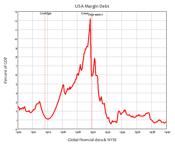
The scale of speculative borrowing when Coolidge was lauding his government’s surplus is staggering: margin debt rose from about 1% of GDP when he came to office to over 12% by the time of the 1929 Crash. It plunged even faster than it rose in the aftermath, to bottom at ½% of GDP in 1933. During the post-WWII period, it remained well below 1% of GDP until the Clinton administration came to power—obsessed, as Coolidge was, with achieving a government surplus.

Figure 36: When governments run surpluses, the private sector gambles

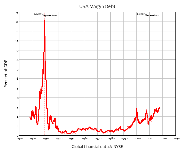
Correlation is not causation, but once again, the level of margin debt rose, from ½% of GDP in 1992 to the Triple Peaks of 2000, 2007, and … now (the data is incomplete because of changes in how it is recorded—whoever designed the latest data set at https://www.finra.org/investors/learn-to-invest/advanced-investing/margin-statistics needs to do some basic courses in data management!).

Figure 37: Margin debt over the long term

The bottom line of this set of posts is that we have to think about finances in an integrated manner, and not just focus upon one component, as “deficit hawks” like Hern do. With an integrated perspective, the sensible conclusion is the one MMT reaches: that the government should run deficits and be in negative equity, to enable the private sector to run surpluses and be in positive equity. Periods of apparent prosperity that coincided with the surpluses of the Coolidge and Clinton eras were the result of private sector levered speculation by a private sector that was experiencing (identical) deficits at the time. Rather than “saving for a rainy day”, these government surpluses helped set off speculative bubbles whose later crashes caused the greatest economic downturns in America’s pre-Covid history.

Private sector deficits are “unsustainable, irresponsible, and dangerous”. Public sector deficits are sustainable, responsible (subject to their impact on inflation and the balance of trade), and safe. It’s time for the “Deficit Hawks” to worry about private sector deficits, not the public sector deficit.

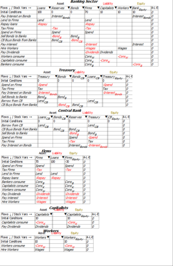
Postscript: The model

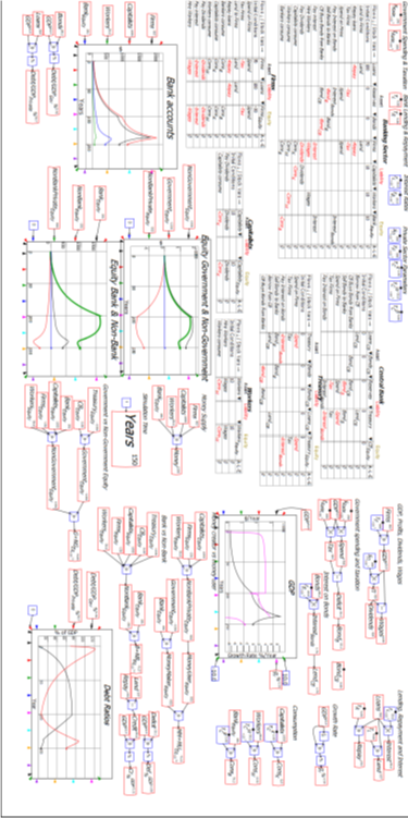
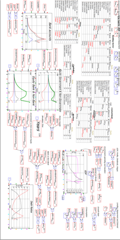
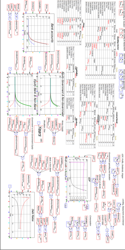
Figure 38 shows the full six Godley Tables that constitute this model, and Equations to show the equations of this model. If you’d like to explore this model yourself (it is attached to this post), download the latest beta release of Minsky from https://sourceforge.net/projects/minsky/files/beta%20builds/. The beta has features used here than are not in the current release version (Version 2.18) and it is very close to being a new release itself. If the release version is later than 2.18 by the time you read this paper, then download the release version instead (unless you feel like being adventurous with the beta).

Figure 38: Full Minsky MMT Model