Background: A record of failure

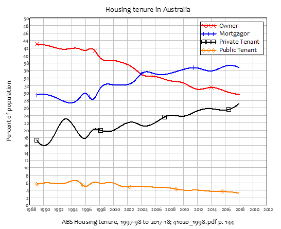
If the objectives of Australian housing policy were to drive house prices out of reach of young Australians, to reduce home ownership, to increase household indebtedness, and to force non-owners onto the private rental market, then it has been a resounding success. Between 1988 and 2018, the proportion of Australians owning their homes outright fell from 43% to 32%; the fraction in mortgage debt rose from 30% to 37%; and the fraction renting from private landlords rose from 18% to 28%—see Figure 1. Many young people, if they can afford to buy a house at all, are forced by high house prices to buy “investment properties” in regional centres, because they can no longer afford to buy a home in the capital cities.

Figure 1: Housing tenure in Australia (smoothed bi-annual data from Census surveys)

Of course, these outcomes were the exact opposite of the intention of government policy, which—regardless of which political party was in office—was to increase home ownership. That these policies have been an utter failure is obvious. At the very least, we need to reverse the effect of these past failures. To do so, we need to understand what these policies were, and what other aspects of housing they affected that led to these disastrous outcomes.

An intergenerational plea

We won’t beat about the bush here: if we are to restore intergenerational equity, then house prices must fall. There is no such thing as expensive affordable housing. The longer the house price bubble goes on, the more the social compacts in this country between rich and poor, young and old, propertied and propertyless, will fall apart.

If you are an older Australian who owns his/her own house, either outright or with a mortgage, you quite possibly have younger relatives who can no longer afford to buy a house in the capital cities, without you risking your equity to help them. Many essential service workers can no longer afford to buy in the cities: an insecure lifetime of renting is their only option. This can’t go on.

But how do we get out of this trap of ever-rising house prices, which benefit the old and the propertied, while impoverishing the young and the propertyless? We certainly can’t do it by a continuation of the policies that got us into this mess.

In this document, we suggest a pair of policies which we believe can pull off the “impossible”. They can reduce house prices, without reducing the equity that older Australians have in their homes—in fact, they can speed up how fast those with mortgages get to be debt-free. They can enable owners without mortgages to realise some of their equity, without having to sell their homes. And they can reduce house prices, to make it possible for would-be homeowners to buy their first homes.

Our first policy actually increases the equity of homeowners and renters alike. Our second reduces house prices, leaving homeowners no worse off than they are now, while substantially improving the situation of would-be homeowners via lower house prices.

If this, at first glance, sounds like magical thinking to you, it’s because past policies have themselves been driven by magical thinking. You need to understand why those policies were wrong—and why they caused this bubble—before we can explain the two policies that can unwind the black magic of the property lobby:

1. A “Monetary Reset”, which reverses the private debt mistakes of the last 30 years; and
2. Rules that limit mortgage debt based on the income-earning potential of the property

Past housing policies: stoking demand and debt

By far the dominant approach, under both Labor and Liberal governments, has been to add to the demand side of the housing market. This has primarily been done by giving grants to first home buyers, but also by encouraging house purchases as investment properties—see Table 1.

Table 1: Australian government schemes to increase house buying power by date and political party

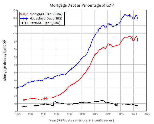
However, these grants and tax credits are only a fraction of the sum needed to purchase a house: the overwhelming proportion of the purchase price comes from mortgage debt. As Figure 2 shows, personal debt has not grown relative to GDP since the 1970s, while mortgage debt has risen almost sixfold since the first of these government interventions in the housing market: the introduction of the “First Home Owners’ Scheme” under Labor Prime Minister Bob Hawke in 1983.

Figure 2: Household debt in Australia

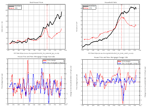
This increase in mortgage debt is the primary cause of higher house prices. Since new mortgage debt is the main source of house-buying power, there is a causal link between rising levels of new mortgage debt, and rising house prices. Figure 3 illustrates this, by comparing the USA to Australia. Everyone acknowledges that the USA had a housing bubble, which burst and caused the GFC. However, many pundits claim that Australia hasn’t had a housing bubble, simply because its house prices haven’t crashed yet. Figure 3 shows that both countries have had, and continue to have, debt-fuelled housing bubbles: they’re just at different stages in the process.

Despite very different trends in house prices (the top left plot) and household debt (top right), the relationship between change in new household debt and change in house prices (Australia bottom left, USA bottom right) is the same: when new household debt is rising, house prices rise, and when new household debt is falling, house prices fall. The key to taming runaway house prices is to tame runaway bank lending.

Figure 3: Australia and the USA: Very different price & debt trends, same causal house price relationship

We also need to extricate ourselves from the impasse that past policies have trapped us in, with house prices and household debt that are both too high. And we need a means to reduce house prices—so that young people who have been priced out of the market can buy in—without bankrupting those who are already in too much debt, and who depend upon high prices to keep themselves in positive equity. We need to do this in a way that will also not cause the financial system to collapse, as it did during the Global Financial Crisis in the USA and Europe.

Finally, we need genuine reforms to bank lending that prevent a house price bubble forming again. We need to encourage bank lending to support building up Australia’s productive capacity and economic resilience, rather than supporting a never-ending speculative bubble.

It is possible to achieve all this, but it can’t be done with the thinking that has led us into this trap, which is shared by both major parties. This thinking is that:

• Government debt is bad, because it borrows money from the private sector that it could otherwise use for investment, and it imposes a burden of debt repayment on future generations; but
• Private debt is simply some individuals lending to other individuals, and its level is easily controlled by varying the interest rate.

These views come straight out of standard economics textbooks. Here’s how they are expressed in Gregory Mankiw’s influential textbook Macroeconomics:

When a government spends more than it collects in taxes, it has a budget deficit, which it finances by borrowing from the private sector or from foreign governments. The accumulation of past borrowing is the government debt… government borrowing reduces national saving and crowds out capital accumulation… Many economists have criticized this increase in government debt as imposing an unjustifiable burden on future generations.…

Saving is the supply of loanable funds—households … deposit their saving in a bank that then loans the funds out. Investment is the demand for loanable funds—investors borrow from the public … by borrowing from banks. Because investment depends on the interest rate, the quantity of loanable funds demanded also depends on the interest rate. (Mankiw 2016, pp. 555-557, 72. Emphasis added)

All these ideas are wrong.

This may seem an outrageous claim to make—surely economists know how money works? However, no less an authority than The Bank of England has said that economic textbooks are wrong about how banks work:

The reality of how money is created today differs from the description found in some economics textbooks:

• Rather than banks receiving deposits when households save and then lending them out, bank lending creates deposits.
• In normal times, the central bank does not fix the amount of money in circulation, nor is central bank ‘multiplied up’ into more loans and deposits (McLeay, Radia et al. 2014, p. 14. Emphasis added)

Economic textbooks are as wrong about how governments operate as they are about how banks operate. We need to explain why they are wrong, before we can explain how it is possible to reduce house prices, maintain the equity that existing homeowners have in their homes, and keep the banking sector solvent.

How government finances actually work

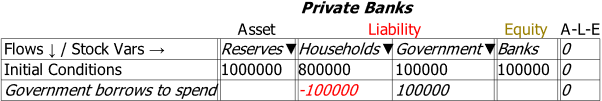
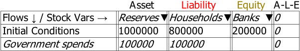
The conventional way of thinking about government is to treat it like just another household. If another household borrows off you, you have less money to spend, and they have more. This way of thinking is shown in Figure 4. If it were correct, then yes, government spending would require first require government “borrowing from the private sector”, and it would “crowd out capital accumulation”.

Figure 4: The wrong, conventional way of thinking of government as “like a household”

However, this model is wrong. Though, like most governments, the Australian Government has accounts at private banks, the Government’s bank is the Reserve Bank of Australia (RBA)—and it is also the bank for private banks. When the government spends, it transfers funds from its RBA account to the accounts of the private banks at the RBA (“Reserves” in Figure 4), and the private banks then credit the deposit accounts of the public.

This actual situation is shown in Figure 5: when the government spends, it credits both the public’s deposit accounts at private banks, and the Reserve accounts of the private banks. Government spending creates money, which turns up in the deposit accounts of the public. Since the government can create money, it doesn’t need to borrow from you—or anybody else—to finance its spending.

Figure 5: The bare bones of the actual situation. The government is a money-creator, not a borrower

In practice, the government is one of two money-creators in the economy:

• The government creates “fiat money” when it spends more than it takes back in taxes; and
• Banks create “credit money” when they lend out more than they take back in repayments.

Government debt is also very different from household debt.

Household debt is mainly in the form of loans secured against household property—”mortgage” is derived from the two French words “mort” and “gage”, meaning “dead” and “pledge”. If you can’t meet the terms of the mortgage, you lose your property. If the bank doesn’t deem you creditworthy (though of course banks have very low standards these days), you can’t get the mortgage. If you don’t get a mortgage, you can’t afford to buy the house. You need the debt before you can do anything.

On the other hand, net spending by government creates money, as Figure 5 shows. The government doesn’t need to borrow to be able to spend. It issues bonds as part of this money-creation process, but this is done, not to raise money from the private sector, but to enable the Treasury to avoid running an overdraft at the Central Bank.

Most countries have passed laws that prevent the Treasury from running an overdraft at the Central Bank. This is a legislative rule: it is not impossible, in an accounting sense, for the Treasury to operate with an overdraft.

Operating with an overdraft—a negative balance on a deposit account—is a difficult thing for a household or firm. The bank might not grant one to begin with, so any transactions that would push your account into the red will be disallowed. If the bank does grant one, it will come with a penalty interest rate—higher than you would pay for an ordinary loan. The bank can also impose onerous conditions on the overdraft which, if they are breached, can send you bankrupt.

A Treasury faces none of these problems, since it owns the Central Bank. Most counties don’t require the Treasury to pay interest to the Central Bank on any bonds that it holds, and even in those where the Treasury is required to pay interest to the Central Bank, Central Bank profits are eventually remitted to the Treasury. Therefore, there is no technical problem with a Treasury overdraft at the Central Bank. But in almost all countries, including Australia, laws force the Treasury to sell bonds to avoid an overdraft.

Here, once more, the Treasury is in a much better situation than a private entity that tries to sell bonds. This is because there is no danger of Treasury bonds not being purchased, regardless of the interest rate offered on them, since they are purchased by the banking sector using Reserves that are created by government spending in the first place: as Figure 5 shows, government spending creating money by adding to the deposit accounts of Households, and it creates additional Reserves for banks as well.

Reserves are an asset of the banking sector which (a) cannot be traded and (b) normally earn no interest. Government bonds, on the other hand (a) can be traded and (b) normally earn interest. When the Treasury offers to sell Bonds to the private banks, it enables the banks to swap non-tradeable, non-income-earning Reserves for tradeable, income-earning Bonds. It is “an offer too good to refuse”, which is one reason that government bond issues are always over-subscribed.

What does the government get out of this transaction? The revenue from selling the bonds to the banks “tops up” its account at the Central Bank, so that the account doesn’t go into overdraft. That, and not “borrowing in order to spend”, is why governments sell bonds when they run deficits.

Whether the government issues bonds or not, if it spends more than it gets back in taxes, then its net financial position will be negative: its financial liabilities will exceed its financial assets.

This might sound horrifying: “How can the government operate in negative equity?!” But in fact, all governments do, including Australia’s. According to the IMF, in 2020, the Australian government’s net financial worth in 2020 was minus $815 billion (see Table 2). This was not an aberration, but the normal situation for Australia (boosted somewhat by Covid), and the normal situation for every national government on the planet.

Table 2: The IMF’s record of Australian government assets and liabilities (https://data.imf.org/regular.aspx?key=61042577)

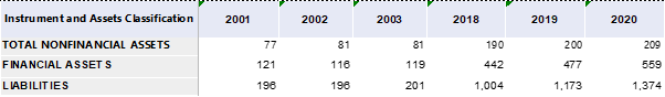
Therefore, the answer to the question “How can the government operate in negative equity?” is “a lot better than you can”. Because the government is both a money creator and “owns its own bank”, not only can it sustain being in negative equity, but its negative equity is what enables you to be in positive equity.

Figure 6 illustrates, in a stylized way, four essential points about how government finances actually work:

• Net government spending—spending in excess of taxation—creates money for the non-bank public, and Reserves for the banking sector;
• Purchases of Treasury bonds by the banking sector convert non-income earning, non-tradeable Reserves into income-earning, tradeable Bonds;
• The government’s negative financial equity—its excess of financial liabilities over financial assets—enables the general public to have positive financial equity—an excess of financial assets over financial liabilities; and
• Bond sales allow this negative financial equity to not show up in the Treasury’s account at the Central Bank (the government’s non-financial assets, however, can be substantial and positive—both in the form of businesses and land that the government owns, and the notional worth of the country that the government administers).

Figure 6: Net government spending creates net financial assets for the non-government sector

The bottom line of this is that the government should normally run a deficit, since that provides the “debt-free” money that a growing economy needs. If it attempts to run a surplus, it necessarily pushes the private sector into a deficit.

The private sector’s response to this is normally to borrow from banks, in order to speculate on non-financial assets—predominantly housing, but also gold, shares on the secondary market, cryptocurrencies, etc. The obsession that both Liberal and Labor governments have had on running a government surplus has helped set off the Australian debt-fuelled housing bubble, and encouraged private sector speculation, rather than private sector enterprise.

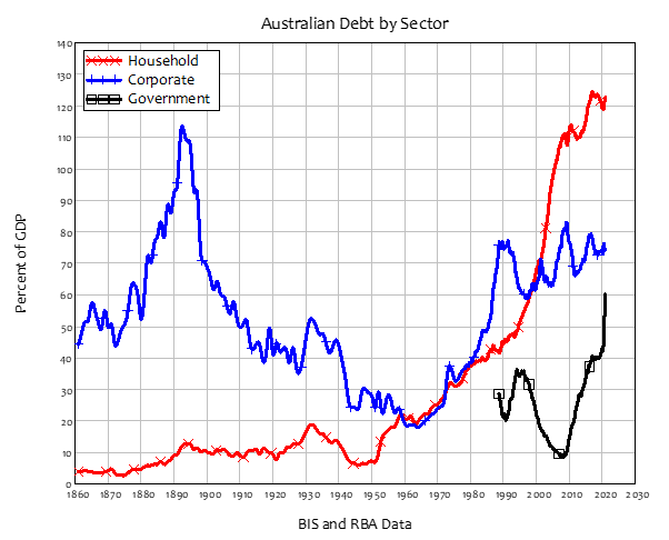
Australia’s debt history

From the focus of both Liberal and Labor parties on the level of government debt, and their lack of discussion of household and corporate debt, you might automatically think that government debt is relatively huge, while corporate and household debt are relatively small. In fact, nothing could be further from the truth. Even after Covid, government debt is less than half the size of household debt, while it is about 10% of GDP less than corporate debt—see Figure 7 (before Covid, government debt was 30% of GDP less than corporate debt).

Figure 7: Australian debt by sector. BIS Data https://www.bis.org/statistics/full_bis_total_credit_csv.zip

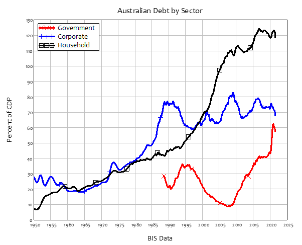
Furthermore, more than 100% of the increase in private debt since 1990 has been from increased mortgage debt: household debt was 45% of GDP in 1990, and corporate debt was 74%; corporate debt in 2021 was 6% lower than in 1990, at 68% of GDP, while household debt was 74% higher, at 118% of GDP. All this additional household debt has done is to inflate house prices.

It was a mistake to let household debt increase at all, let alone this much—tripling compared to GDP in just over 30 years. This mistake must be reversed. With an understanding of how money is created, it is possible to reverse it, by replacing bank-debt-based money with government-fiat-based money. This can be done in a way that:

• makes it possible for house prices to fall, without reducing the equity of existing homeowners and mortgagors; and
• does not benefit those who rode the housing bubble at the expense of those who did not.

We need a monetary reset that will convert debt-based money to fiat-based money, and unwind this historic mistake.

A Monetary Reset

The monetary reset would:

• Give every Australian adult an identical sum of government-created money;
• Require those who had debt to use that money to pay down their debt;
• Sell Treasury Bonds to banks, precisely as is currently done in deficit financing; and
• Require individuals with less debt than the amount issued to purchase Treasury Bonds from banks, from which they will earn interest income;
• This would not create any additional money and put inflationary pressure on the economy, but rather, it would change the asset backing the money from private debt, to reserves and government bonds;

The essential steps in the monetary reset are shown in Figure 8:

• Create fiat money for the public and reserves for the banks;
• The public repays much of its private debt;
• Banks buy bonds with the reserves created by the reset;
• Banks are paid interest on their bonds; and
• The RBA buy bonds from the banks;

Figure 8: The essential steps in the monetary reset

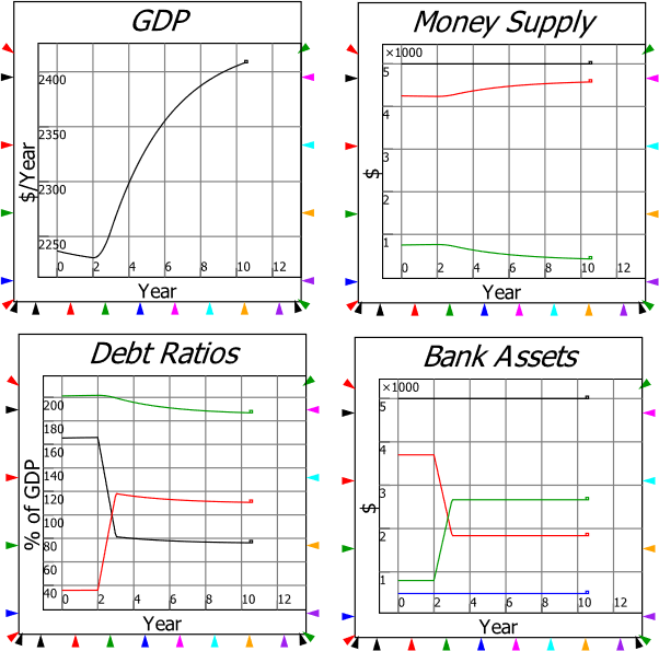
The outcomes of the monetary reset are:

• A dramatic and necessary fall in the indebtedness of the Australian public;
• A matching increase in the public’s financial equity. The pressure to speculate to achieve financial security for your future is substantially reduced;
• An increase in GDP, as money is redistributed away from the finance sector and towards the real economy; and
• A fall in the total debt ratio, as the private debt ratio falls more than the government ratio rises

Figure 9: A simple simulation of a monetary reset. See Appendix for full details

This policy on its own will reverse the mistake of the last 30 years of feeding the housing bubble, and it actually increases the net equity position of homeowners, as well as those who are currently renting. But it doesn’t necessarily reduce house prices. That is the role of our next policy.

Property Income Limited Leverage

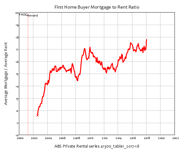
The current ratio of the average mortgage to the average rent in Australia is of the order of 20 to 1—see Figure 10, which has data up to 2018 (the ratio has surely gotten worse with the bubble that has occurred during Covid). As little as 20 years ago, it was of the order of 10 to 1. This is what has made entry into the housing market impossible for the young: though interest rates have fallen, the deposit needed to enter the market has risen far faster than incomes, and even faster than house prices themselves.

This is irresponsible lending—something that the Morrison Government has actively encouraged by its outrageous reactions to the findings of the Banking Royal Commission. We are going to bring irresponsible lending to an end.

We will introduce a law limiting the maximum amount that can be lent to buy a house to a multiple of its rental income. Initially this will start near the current ratio, but the ratio will be progressively reduced until the maximum amount that can be borrowed to buy a property will be ten times its annual rental income. So if a house would rent for $1000 a week, the most that could be borrowed to buy it, by anyone, would be $520,000.

By reducing the amount of debt that can be used to buy a property, this policy will reduce house prices. It would also mean that, if two parties were vying for the same property, the one that raised more money via savings would win. It will stop us rewarding leverage and start rewarding frugality as the first step towards home ownership.

Figure 10: Ratio of average first home mortgage to average rent

On its own, this policy would benefit house buyers and penalize house sellers. This is why we have paired it with a Monetary Reset, which, on its own, increases the equity of homeowners and renters equally. The policy objective we have—which will be difficult but not impossible to achieve—is to offset the two policies, so that homeowners end up no worse off, while renters benefit so that the property and intergenerational unfairness of the last 30 years is reversed.

Existing homeowners would therefore retain the benefits they have gained from 30 years of bad policy and the housing bubble it allowed. The primarily young people—but also low-income older Australians—whom those policies discriminated against would benefit from both of our policies, via increased financial net worth from the Monetary Reset, and a fall in house prices to bring them back into line with incomes.

Conclusion

The policies outlined in this document are undoubtedly radical and untested. But the conventional policies that have been followed by both major parties have been tested and have clearly failed. It is time to try something new.

Technical Appendix

Modelling a Monetary Reset

The model in this document is constructed in the Open Source system dynamics program Minsky (see https://sourceforge.net/projects/minsky/), which has been designed to enable monetary systems to be modelled easily. It uses double-entry bookkeeping—the accountant’s “Graphical User Interface”—to ensure that models are correctly structured.

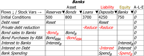
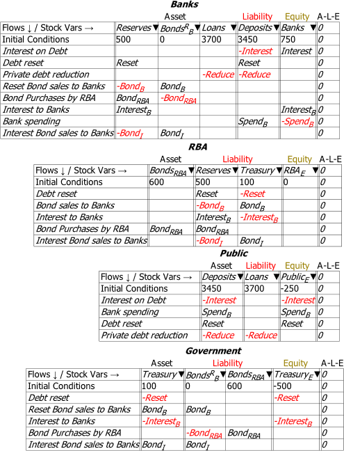
This simplified model does not distinguish the public into separate groups—homeowners, mortgagors, renters. It therefore doesn’t divide private debt into its key components—mortgages, unsecured household debt, and corporate debt. Its purpose is to illustrate the key operations in a Monetary Reset, and how they interact. These key operations are shown in Figure 12, which shows the banking sector’s views of the operations involved in what is known as a “Godley Table”.

Figure 11: The essential operations in a monetary reset

The operations are, reading down the rows:

1. The public pays interest on the existing level of private debt;
2. The debt reset occurs, with an injection of money into the public’s deposit accounts, and an identical injection of reserves into the banking sector’s Reserve accounts at the RBA;
3. The public reduces it debt level using the monetary reset;
4. Bonds equivalent in value to the Reset are sold to the private banks, who purchase them using the Reserves created by the Reset;
5. More bonds are sold, equivalent in value to the interest on the bonds;
6. The RBA optionally purchases bonds from the private banks;
7. Interest payments on the bonds are made to the banks; and
8. The banking sector hires staff, and buys goods and services, from the non-bank private sector.

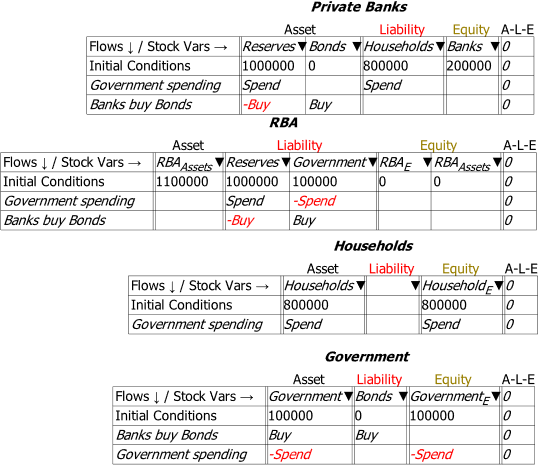
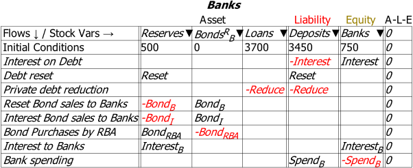
The main purpose of this model is to show that a Monetary Reset is feasible: the accounting works. Figure 13 shows all the Godley Tables in the model: the banking sector (the same as in Figure 12); the RBA; the non-bank Public; and the Government.

Figure 12: All “Godley Tables” in the model

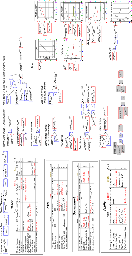
The full model is shown in Figure 14.

Figure 13: The complete simple model of a Monetary Reset

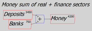
The model is defined using flowcharts. For example, the money supply is defined as the sum of the deposits of the public at private banks (“Deposits”) and the short-term equity or operating accounts of the banks (“Banks”)—see Figure 15:

Figure 14: Definition of money

GDP is defined as the turnover of money in the “real” economy—the deposits of the private non-bank public:

Figure 15: GDP from turnover of money in the non-bank public’s bank accounts

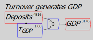
The parameter is what is known in engineering as a “time constant”. It tells you how many years it would take for something to turn over completely. The value 1.6 here means that the money supply would turn over completely in 1.6 years. This value was chosen so that the GDP of this toy model began at Australia’s current GDP of roughly $2200 billion (the model’s starting value for GDP is $2156 billion, compared to the $2194 billion figure recorded in July 2021).

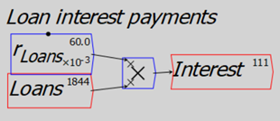
Interest equals the rate of interest on bank loans times outstanding loans:

Figure 16: The simplest equation in the model. Interest payments equal the rate of interest times outstanding loans

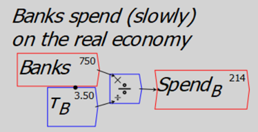
Banks then spend their share of the money supply on the “real” economy. The turnover rate is 3.5 years, to reflect the fact that the finance sector spends more slowly on the real economy than the real economy does on itself.

Figure 17: Banking sector spending on the real economy (salaries, buying goods and services, etc.)

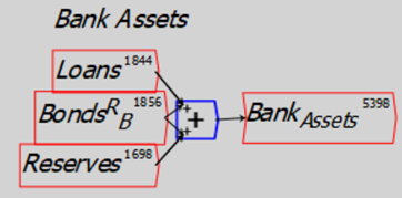
The banking sector earns income from the assets that it owns: it is paid interest on loans by the private sector, on its bond holdings by the government, and normally earns no income on its reserves.

Figure 18: Bank Assets

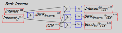
The next flowchart sums the two interest flows into bank income, and calculates the ratio of these income flows to GDP.

Figure 19: Bank income from interest, plus calculating some ratios

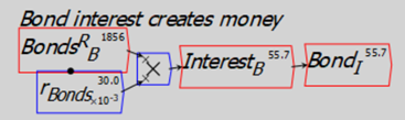
The next flowchart is where things start to get slightly complicated. The first part of it shows that interest on bonds equals bonds held by the banks times the rate of interest on bonds; the second shows that the government issues more bonds to cover this interest payment. This happens because there are laws stopping the Treasury from simply borrowing this amount—at no interest—from the RBA.

Figure 20: Interest on Bonds creates money, and more bonds are issued to cover the interest bill

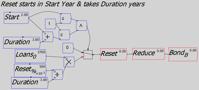
The next bit is the most complicated part of the model. It says that the Reset starts in year (which is set to year 2 in this simulation) and lasts for years (which is set to 3 years—in other words, the Reset is a gradual process, rather than all at once). Then the amount created by the government ( dollars per year) is used to private debt, and the government sells the same value of bonds per year
to the banks.

Figure 21: The Monetary Reset starts in “Start” Year and runs for “Duration” Years–Year 2 and 3 years in this simulation

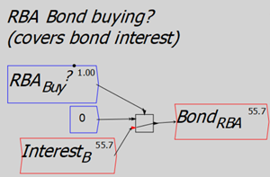
Finally, the RBA can decide whether it buys bonds from the private banks equivalent in value to the interest payments on the Reset bonds.

Figure 22: A policy control setting for whether the RBA buys bonds equivalent to the interest on Reset Bonds

We now run four simulations with the model:

1. No interest is paid on Reset Bonds
2. Interest is paid at 6%, and the RBA buys no bonds
3. Interest is paid at 6%, and the RBA buys bonds
4. Interest is paid at 3%, and the RBA buys bonds

The preferred situation, as we will demonstrate, is the last one: 3% interest on bonds, and the RBA buys bonds from the private banks that are equal in value to the interest paid on those bonds.

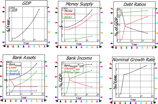
Simulation 1: No interest on bonds

In this simulation, GDP increases, even though the money supply remains constant, because the Reset shifts the distribution of money away from the finance sector and towards the real economy, where money turns over more rapidly. Total debt—the sum of private debt and government bonds—falls relative to GDP. Private debt falls substantially, while government debt rises, but by less than the increase in private debt. Bank income falls substantially as non-income-earning government bonds replace income-earning private debt.

Figure 23: Simulation 1. No interest on Reset bonds

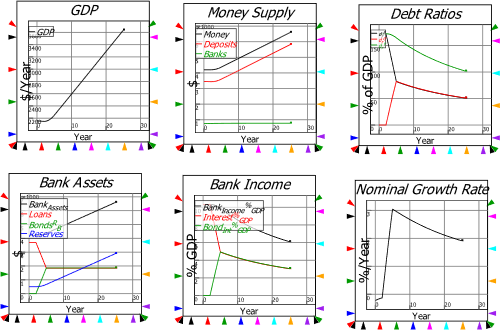
Simulation 2: Bonds pay 6% interest, and the RBA buys no bonds

In this simulation, bonds pay the same rate of interest as the private debt they replace, while the RBA sits on its hands. Now, since the interest is credited to the Reserve accounts of Banks as well as to their short-term equity accounts, the interest payment (a) creates money and (b) creates the reserves the banks need in order to buy the bonds. The GDP therefore grows—but at an increasing rate, because the bonds needed to pay the interest compound at a rate of 6% per year. The nominal growth rate therefore accelerates with the accelerating money supply.

Clearly this is an undesirable situation—but as the next section shows, this is easily prevented if the RBA buys the bonds used to finance the interest on bonds in the secondary market.

 

Figure 24: Simulation 2: 6% interest on Reset Bonds & RBA does not buy interest-covering bonds from the private banks

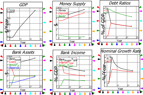
Simulation 3: 6% interest, RBA buys bonds

With the RBA buying the interest-financing bonds, the money creation effect does not compound. GDP grows but at a linear rate, while the nominal rate of growth falls as the effect of the monetary reset fades.

Figure 25: Simulation 2: 6% interest on Reset Bonds & RBA buys interest-covering bonds from the private banks

Simulation 4: 3% interest, RBA buys bonds

Bankers were not always regarded as “Masters of the Universe”: at one point, the best they could manage was “Masters of the golf course”. That is the world of tranquil finance that we would like to re-create. We need more real engineers, and fewer financial engineers.

In this simulation, the interest rate on bonds is 3%, while the rate on loans is 6%. The lower return on bonds is justified because there is no risk to the banks in government bonds—whereas there is some risk in private debt.

The runaway inflationary dynamic of the 2^nd simulation is eliminated by the RBA buying the bonds issued to finance the interest on bonds from the banks in the secondary market. This may appear to be a ruse—and it is, because of the laws most countries have passed to prevent the Treasury borrowing directly from the Central Bank. The purchase of Treasury Bonds from the private banks by the Central Bank achieves the same outcome, albeit with an obvious absurdity of issuing bonds to finance the interest on bonds.

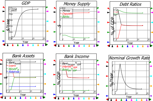
Notice that in this simulation, numerous desirable outcomes occur: debt ratios fall, both in total and separately for both private and government debt. Bank assets rise, and though bank income falls as a proportion of GDP, it comes with a substantial fall in risk as well. Finally, the growth spurt from the Reset stabilizes over time.

Figure 26: The preferred policy: 3% interest on bonds, RBA buys the interest-covering bonds from the private banks

This is our preferred policy setting. Banks should not receive the same rate of interest on bonds as they get on private loans, because the latter carry the risk of the default, while the former do not. This policy also leads to the outcome that banks cease being “Masters of the Universe”, and once again become what they were known as during the 1950s: “3-6-3 businesses: borrow at 3%, lend at 6%, and be on the golf course by 3pm”. An explicit aim of The New Liberals is to return the banking sector to the role it had in the 1950s, of being the servant of the industrial sector rather than its master.

Very Technical Appendix

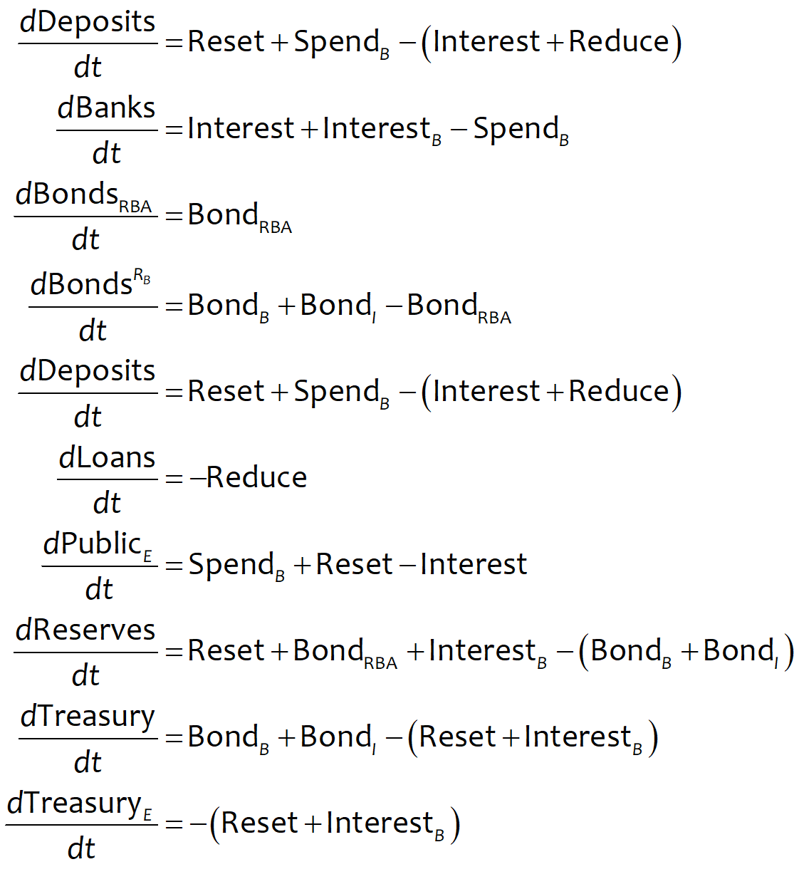
The system dynamics program used in this document is called Minsky. It works by generating systems of differential equations from the flowchart relations shown in the previous section. These equations are shown below, for those who are curious about how the mathematical model used in this document operates.

Minsky is Open Source and can be downloaded from https://sourceforge.net/projects/minsky/.

Differential Equations

        

Initial Conditions

        

 

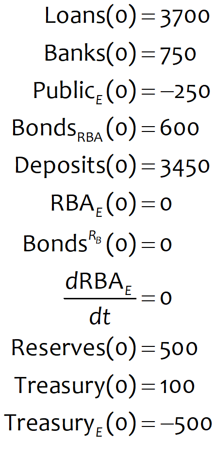
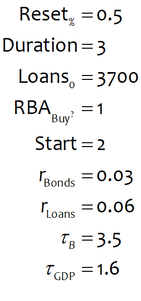
Key Parameters

        

Variables

        

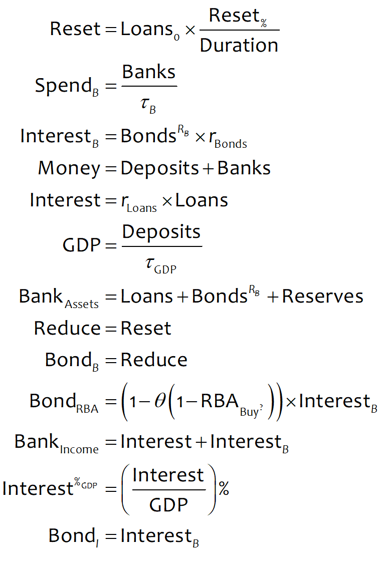
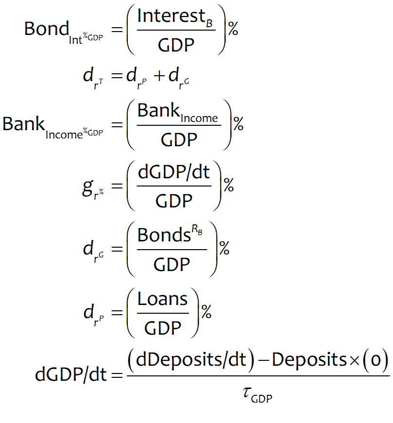
Useful ratios, etc.

        

Australia’s long term debt history

The American philanthropist Richard Vague’s magisterial review of the last one and a half centuries of economic crises (Vague 2019) found that all of them had been caused by the collapse of private debt bubbles. This has also been Australia’s long term history of private debt, which is well described in the RBA publication Two Depressions, One Banking Collapse (Fisher and Kent 1999), which compares the 1890s Depression, which was devastating for Australia, to the 1930s, which was relatively mild—though still a Depression.

Figure 27: The long-term history of Australian debt. Private debt has always been the problem

Government balance sheet

Like almost all governments, the Australian government has always been in a net negative position in terms of financial assets—assets which are a claim on other parties—because that is the flipside of other parties—the private sector—being in net positive equity.

The data source is https://data.imf.org/regular.aspx?key=61042577.

Figure 28: Financial Assets & Liabilities in A$ billions

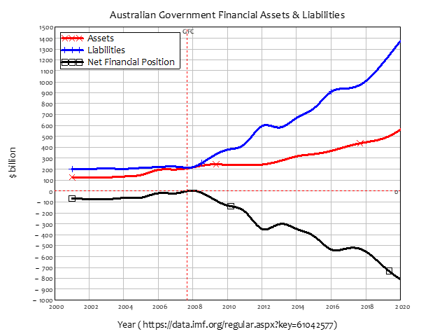
Notice that the GFC coincided with Australia achieving a net zero position on government net financial assets and liabilities. As we argue in the body of this policy document, this “achievement” was a mistake that contributed to the excessive level of private sector financial speculation.

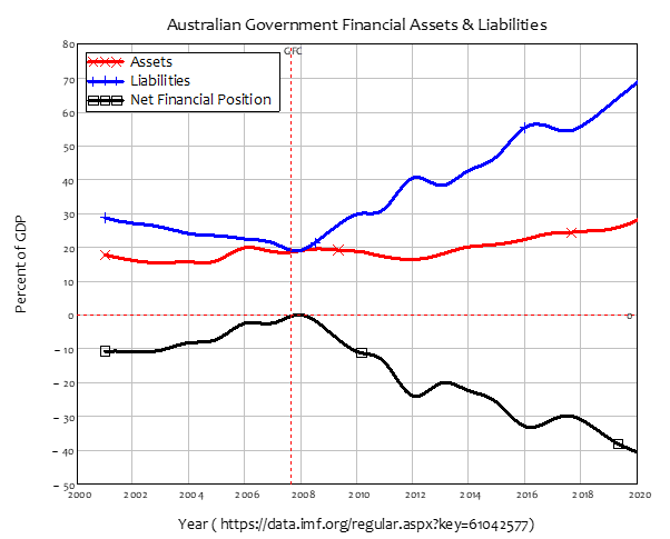
Figure 29: Assets and Liabilities as Percent of GDP

References

Fisher, C. and C. Kent (1999). Two Depressions, One Banking Collapse. Reserve Bank of Australia Research Discussion Papers. Sydney, NSW, Australia, Reserve Bank of Australia. 1999: 54.

Keen, S. (2021). The New Economics: A Manifesto. Cambridge, UK, Polity Press.

Kelton, S. (2020). The Deficit Myth: Modern Monetary Theory and the Birth of the People’s Economy. New York, PublicAffairs.

Mankiw, N. G. (2016). Macroeconomics. New York, Macmillan.

McLeay, M., A. Radia and R. Thomas (2014). “Money creation in the modern economy.” Bank of England Quarterly Bulletin
2014 Q1: 14-27.

Vague, R. (2019). A Brief History of Doom: Two Hundred Years of Financial Crises. Philadelphia, University of Pennsylvania Press.