I’ve been focusing on the economics of climate change for over four years now, because it’s the most pressing problem facing humanity, and because economists have done such a god-awful job on it—fooling themselves into regarding an existential threat as a minor cost-benefit problem (Keen 2020; Keen et al. 2022).
For circumstantial reasons, I can’t do much on this topic right now, and rather fortuitously, I received this email earlier this week:
I am a massive fan of your work, and I would like to take this opportunity to congratulate you for all that you do in the field of economics.
I am recent convert to Keynesian economics having made the shift from the Austrian school of thought.
Just out of interest what is the difference between your variant of Keynesian economics, namely, Post-Keynesian and standard Keynesian/Neo-Keynesian/New-Keynesian?
Wow. This made that correspondent a rarity: most people who begin with Austrian economics, or convert to it, never escape it. He deserved an extended reply, which I gave by email. This is an even more extended commentary on the weird menagerie of schools of thought in economics.
The labels that macroeconomists use to describe themselves are a recipe for confusion, which in turn mirrors the confusion of the ideas behind them. As I wrote my reply, I reached the conclusion in the title, that Keynesian Economics was doomed within the mainstream of economics from one year before
The General Theory was published.
Equilibrium arising from a failed attempt at dynamics
Standard “Keynesian” economics began with the IS-LM model, which was introduced by John Hicks in his paper “Mr Keynes and the Classics—a Suggested Interpretation” (Hicks 1937). This model portrayed Keynes’s macroeconomics using a diagram with two intersecting curves, one representing investment and savings (hence “IS”), the other representing liquidity and money (hence “LM”—though Hicks initially used the initials “LL”). The intersection of the two curves jointly determined both the level of economic activity (on the horizontal axis) and the interest rate (on the vertical).
Figure 1: Hicks’s first drawing of the IS-LM model (Hicks 1937)
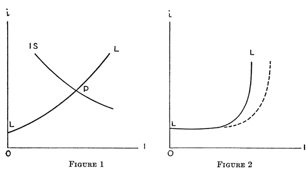
The IS curve was like the microeconomic demand curve, and the LM was like the microeconomic supply curve, so this way of interpreting Keynes put Neoclassical economists back on familiar territory. Many had never even read Keynes’s original General Theory of Employment, Interest and Money (Keynes 1936), while those that did simply failed to understand it. Robert Lucas, the “Nobel Prize” winner who was a major architect of the “New Classical” approach, put it this way in 2003:
I’m going to think about IS-LM and Keynesian economics as being synonyms… I asked my colleague [another “Nobel Prize” winner] Gary Becker if he thought Hicks had got the General Theory right with his IS-LM diagram. Gary said, “Well, I don’t know, but I hope he did, because if it wasn’t for Hicks, I never would have made any sense out of that damn book.” That’s kind of the way I feel, too, so I’m hoping Hicks got it right. (Lucas 2004)
Hicks didn’t get it right: he found Keynes as incomprehensible in the 1930s as Lucas did in the 1980s. What Hicks did instead, when charged with writing a book review of The General Theory, was to present an idea he first thought of in 1935—”before I wrote even the first of my papers on Keynes” (Hicks 1981)—as an interpretation of Keynes.
This is an endemic problem in economics, which makes trying to follow its history like trying to unravel a game of Chinese Whispers: only by reading the whole canon can you actually work out what the hell went wrong. In this case, “Keynesian Economics” went wrong even before the publication of The General Theory, when Hicks failed in a grand ambition to build a dynamic model of a monetary production economy.
In a paper called “Wages and Interest: The Dynamic Problem” (Hicks 1935), Hicks attempted to model an economy which produced a single commodity—bread—using inputs of labour and machinery (“Capital”). His sticking point was that he couldn’t work out how to make machinery out of bread:
For the entrepreneur has actually to determine, not only how much labour he will employ in the first week, but how he will employ that labour, whether in the production of bread for the next market day, or in the production of bread for the more distant future (activity which, a week after, will only have resulted in the production of equipment). (Hicks 1935)
Huh? How does stale bread become “equipment”? Hicks couldn’t work out how—and I genuinely sympathize with his dilemma, because I later solved this problem in as-yet-unpublished work with Matheus Grasselli and Tim Garrett (see https://www.patreon.com/posts/correcting-on-of-63360796 and https://www.patreon.com/posts/one-for-nerds-of-39055598), and it wasn’t easy (I outline my solution later in this post).
Unfortunately, in the middle of his paper, Hicks changed tack from a dynamic model to an equilibrium one—and ultimately, IS-LM was born. Though he couldn’t work out how to complete his dynamic model, he reasoned that he could model the equilibrium of a three-market system with only two markets, because:
if the market for labour is in equilibrium, and if the market for bread is in equilibrium, the market for loans must be in equilibrium too. (Hicks 1935)
This is applying “Walras’ Law”. As Hicks explained:
The reason why we can refer back to the bread market in this way is that we have taken bread as our standard of value. There are two prices to be determined—a rate of wages and a rate of interest; and three equations to determine them—equations of supply and demand for labour, loans and bread. Of these three equations (as in the system of Walras) one follows from the other two. But it is completely indifferent which of the three equations we strike out in this way; convenience seems to dictate that we should strike out the equation relating to loans. (Hicks 1935)
Hicks’s IS-LM model did the same thing:
the idea of the IS-LM diagram came to me as a result of the work I had been doing on three-way exchange, conceived in a Walrasian manner. I had already found a way of representing three-way exchange on a two-dimensional diagram… Keynes had three elements in his theory… The market for goods, the market for bonds, and the market for money: could they not be regarded in my manner as a model of three-way exchange? In my three-way exchange I had two independent price parameters: the price of A in terms of C and the price of B in terms of C (for the price of A in terms of B followed from them). These two parameters were determined by the equilibrium of two markets, the market for A and the market for B. If these two markets were in equilibrium, the third must be also. (Hicks 1981. Emphasis added)
Hicks later realized that what he had done was a distortion of Keynes—and he explained why in a paper entitled “IS-LM: An Explanation” (Hicks 1981) that I think of as “IS-LM: An Apology”. A key problem was getting rid of the third market by assuming that the other markets were in equilibrium.
For starters, this neuters the key problem that Keynes was focusing on: how do you reduce the huge level of involuntary unemployment during the Great Depression, when at its peak, 25% of the US workforce was out of work? Surely the labour market was not in equilibrium.
Secondly, even in the guise of Hicks’s IS-LM diagram, equilibrium only applied at one point—where the IS and LM curves intersected. The IS curve was supposed to show all the combinations of the level of economic activity and the interest rate that put the goods market in equilibrium; the LM curve showed all the combinations that put the money market in equilibrium; but only at the point where the two curves intersected were both the goods market and the money market in equilibrium, and therefore only at that point could the labour market also be in equilibrium, according to Walras’ Law—and therefore be ignored. Outside of this point—that is to say, across the whole space of the IS-LM diagram—at least one of the goods (IS) or money (LM) market must be out of equilibrium, as must also be the labour market that the IS-LM diagram omitted.
Hicks himself realized this in the 1970s. Only the point of intersection of the two curves could be seen as a point of “general equilibrium” as assumed in Walras’s Law. At the same time, it was impossible to treat this point as a description of the real economy at critical times in the economy’s development, such as the most recent economic crisis Hicks had experienced in 1975:
Applying these notions to the IS-LM construction, it is only the point of intersection of the curves which makes any claim to representing what actually happened (in our “1975”). Other points on either of the curves—say, the IS curve—surely do not represent, make no claim to represent, what actually happened. They are theoretical constructions, which are supposed to indicate what would have happened if the rate of interest had been different. It does not seem farfetched to suppose that these positions are equilibrium positions, representing the equilibrium which corresponds to a different rate of interest. If we cannot take them to be equilibrium positions, we cannot say much about them. But, as the diagram is drawn, the IS curve passes through the point of intersection; so the point of intersection appears to be a point on the curve; thus it also is an equilibrium position. That, surely, is quite hard to take. We know that in 1975 the system was not in equilibrium. (Hicks 1981)
Hicks’s conclusions about IS-LM were quite brutal—and quite justified:
I accordingly conclude that the only way in which IS-LM analysis usefully survives—as anything more than a classroom gadget, to be superseded, later on, by something better—is in application to a particular kind of causal analysis, where the use of equilibrium methods … is not inappropriate…
When one turns to questions of policy, looking toward the future instead of the past, the use of equilibrium methods is still more suspect… It may be hoped that, after the change in policy, the economy will somehow, at some time in the future, settle into what may be regarded, in the same sense, as a new equilibrium; but there must necessarily be a stage before that equilibrium is reached. There must always be a problem of traverse. For the study of a traverse, one has to have recourse to sequential methods of one kind or another. (Hicks 1981)
By “traverse”, Hicks meant “change out of equilibrium”, which he thought would lead to a new equilibrium. This is mistaken, given what we know about genuine dynamic systems today: complex systems can and normally do remain “far from equilibrium” forever (Lorenz 1963). But to give him his due, Hicks finally realised that his turn from dynamic methods to equilibrium in 1935 was a mistake.
Unfortunately, Hicks’s revelations occurred forty years after he set off the juggernaut that became “Standard Keynesian” macroeconomics, and none of the wisdom that Hicks displayed here affected Neoclassical economists. Just as most Neoclassicals never read Keynes (and where they did, they made a hack of it), virtually no Neoclassicals have read Hicks’s recantation of IS-LM (certainly not Paul Krugman, the main champion of IS-LM thinking today).
So “standard Keynesian economics” is actually Neoclassical economics, but since it purported to come from Keynes instead, it set off two separate fissures:
- Neoclassicals in general adopted IS-LM as a cut-and-paste onto their standard microeconomics, in what became known as the “Keynesian-Neoclassical synthesis“, developed by Paul Samuelson. So, a more accurate term for “Keynesian Economics” is actually “Samuelsonian Economics“. However, Neoclassical purists always regarded this as an unhealthy graft, and desired instead to derive macroeconomics directly from microeconomics—from “first principles” in their minds; while
-
Economists who actually did understand Keynes regarded the IS-LM model as an abomination, and set out to develop a new economics from what they saw as Keynes’s true foundations, which weren’t microeconomic at all (let alone Neoclassical microeconomic), but:
- the acknowledgement of genuine uncertainty about the future as the core source of macroeconomic instability; and
- the role of money in the light of that uncertainty.
The Neoclassical Menagerie
The first fissure led to standard “Keynesian” macro–IS-LM, AS-AD models etc., basically the stuff that liberal-mainstreamers like Krugman, Mankiw, Summers etc. throw up. The desire by hardcore Neoclassicals to get away from the IS-LM model led to the development of the “New Classical” School of economics by hardcore Neoclassicals—Sargent, Kydland, Prescott, Lucas etc.—who were intent on deriving macroeconomics directly from microeconomics:
Nobody was satisfied with IS-LM as the end of macroeconomic theorizing. The idea was we were going to tie it together with microeconomics and that was the job of our generation. (Lucas 2004)
These self-described “New Classicals” built their microeconomic-based macroeconomics using the economic growth model developed by Frank Ramsey in the 1920s (Ramsey 1928). Ramsey’s model described the entire economy as a single utility-maximising entity, balancing the returns from work against the disutility of work, to reach an ultimate goal which he described as Bliss:
What we have in the several cases called the maximum obtainable rate of enjoyment or utility we shall call for short Bliss or B. And in all cases we can see that the community must save enough either to reach Bliss after a finite time, or at least to approximate to it indefinitely. (Ramsey 1928)
In what is a common phenomenon for Neoclassical economics, Ramsey found that this future point of Bliss was mathematically unstable! Geometrically, the dynamics of this point looked like a horse’s saddle, which is stable in one dimension, but unstable in another.
Seen from along the horse’s spine, a saddle is stable: if you dropped a ball on the front or back of the saddle from this perspective, it would ultimately come to rest at the lowest point of the saddle along the horse’s spine. But seen from the side of the horse, the saddle is unstable: if the ball deviated even slightly from the exact centre of the horse’s spine, it would rapidly fall off the saddle. The only way to throw a ball onto a saddle and have it stay there would be move to a point perfectly in line with the horse’s spine, and throw the ball from there with infinite accuracy.
These hardcore Neoclassicals made a virtue of this vice by assuming that “rational agents” could indeed do this, in what they described as “Real Business Cycle” models (RBS). The location of the saddle in space was a function of both individual preferences (the consumer side of the economy) and the costs of production (the firm side of the economy). “Shocks” to both tastes and technology would move the location of the saddle, and “rational agents” would instantly work out where the new Bliss point was. They would then instantly “jump” from where they were—in terms of consumption and production now—to a new location which was on the line drawn from the future Bliss point back to today.
This “jump” would appear as a change in the employment rate and a change in output—the “business cycle”, and this would be a utility-maximizing, equilibrium thing: though unemployment might rise, it did so because this maximized the economy’s utility. This was applied even to the Great Depression, which was described as a utility-maximizing response to unspecified changes in economic policy:
From the perspective of growth theory, the Great Depression is a great decline in steady-state market hours. I think this great decline was the unintended consequence of labor market institutions and industrial policies designed to improve the performance of the economy. Exactly what changes in market institutions and industrial policies gave rise to the large decline in normal market hours is not clear…
The Keynesians had it all wrong. In the Great Depression, employment was not low because investment was low. Employment and investment were low because labor market institutions and industrial policies changed in a way that lowered normal employment. (Prescott 1999)
The rising stars of the Neoclassical mainstream (Woodford, Blanchard, etc.), who weren’t as completely detached from reality as Kydland, Prescott and friends, couldn’t stomach the outcome of these models, but they couldn’t fault their methods either: they also thought that macroeconomics should be derived from microeconomics.
Their solution was to use the microeconomics of imperfect competition. They conceded that if perfect competition applied, the macro-outcome would be as the hardcore Neoclassicals described it—full employment. But because of imperfect competition, there would be wage and price “stickiness”. Exogenous shocks would always be disturbing the economy from full employment equilibrium, and because of imperfect competition (in part, but not all, of the economy), the price mechanism would be unable to do its thing and absorb any shock with a change in prices. Because of this “stickiness”, negative shocks to the economy would result in extended periods of involuntary unemployment. This resulted in DSGE models, which are the DNA of the so-called “New-Keynesians“.
They were pretty pleased with themselves when they developed these models—they really thought that they now understood the macroeconomy, because they could fit these models to data just by tweaking their many parameters.
And then along came the GFC, and blew it all away.
The Post-Keynesian Umbrella
The second fissure led to the development of “Post-Keynesian Economics“. This has had its divisive moments and many offshoots, but a fundamental driver has been an emphasis upon realism, and that has overcome any divisive tendencies in the end—though there hasn’t yet been a grand fusion. The threads that dominate it today are Stock-Flow Consistent modelling (derived from the work of Wynne Godley) and Modern Monetary Theory (derived from insights from Warren Mosler, refined by Randy Wray, Bill Mitchell, extended and popularised by Stephanie Kelton, etc.), and there are also substantial subgroups working on complex systems, dynamic modelling, Hyman Minsky’s “Financial Instability Hypothesis” (my main areas).
There’s also other less well-known threads which were dominant at various times in the last century—”Sraffian Economics” (focusing on the input-output nature of production), “Kaleckian Economics” (based on the work of Polish engineer turned economists Michal Kalecki, who developed many of Keynes’s insights by applying engineering thought to economic issues).
Finally, there’s some innovation coming from outside economics that is readily adopted by Post-Keynesian economics. I’d especially single out the work of the mathematician Ole Peters, which he describes as “Ergodicity Economics“: https://ergodicityeconomics.com/. This is actually a bit of a misnomer, since the economy as Peters describes it is a non-ergodic system (technically, a system where the time average of variables is not the same as the space average, whereas mainstream Neoclassical economics pretends that the economy is ergodic).
So, coming across from Austrian economics, there is a lot for you to learn! I tried to create a synthesis of sorts in my recent book The New Economics: A Manifesto (https://www.amazon.co.uk/New-Economics-Manifesto-Steve-Keen/dp/1509545298) but you should also read some history. For a positive history—in that it shows how a decent economics can be constructed, as well as critiquing the failure of Neoclassical economics—I’d recommend Blatt (1983). Dynamic economic systems: a post-Keynesian approach (Blatt 1983). My Debunking Economics (Keen 2001) is also a comprehensive guide to the imbroglio that is modern economics.
My solution to Hicks’s “bread” dilemma
If only Hicks had got it right in 1935, and actually managed to build the dynamic model to which he aspired, maybe IS-LM would never have happened—and economics would be in a far better state. But as the great philosopher Rafael Nadal once put it, “If, If, If? It doesn’t exist“.
The source of Hicks’s dilemma was the common abstraction in economics of a single commodity economy. Any model which has just “GDP” as its output is implicitly assuming that there is a single commodity that can function as both a consumer good and an investment good: the part of it that is eaten is Consumption, the part that is added to the Capital stock of the economy is Investment. But there is no such thing.
Another way to think about these models is that the output is corn—something that can be both eaten now, or stored in a barn to later be planted to yield yet more corn. But this eliminates economics and the system of production from consideration, because nature does everything: no machines are needed, and what is saved is automatically invested (after a time lag as seed corn in the barn). The “Holy Grail” that Hicks sought was to be able to describe the systems of distribution and production—and that included the mechanisms needed to transform the generic commodity from a consumption good into an investment one.
I had originally thought that, to pull off what Hicks had attempted, you would need at least a two-commodity model—one for consumption, the other for investment. But when Matheus Grasselli and Tim Garrett and I attempted to model production using both energy and matter as essential inputs, Matheus insisted that we try to produce a single commodity model, to fit in with the economic convention.
I then found myself staring at Hicks’s 1935 dilemma: how can you make capital equipment out of bread? You can’t. I genuinely felt for him.
But then I remembered the The Iron Giant—a novel and ultimately animated cartoon in which an alien robot, made of iron, crash-landed on Earth just after the Russians launched Sputnik.
 The thought occurred to me that, rather than using a realistic consumption good (bread) with no imaginable investment good (stale bread???), why not imagine a world where an unrealistic consumption good exists (iron, eaten by the workers on the Planet of the Iron Giants), which can also be a realistic investment good (iron, made into blast furnaces, rolling mills, and mining equipment to mine both iron ore and coal)?
The ruse worked, and it generated a model which would have surprised Hicks, had the same idea occurred to him: the equilibrium was unstable, but rather than breaking down, as Hicks falsely believed that unstable systems would do, it generated permanent cycles. It was another manifestation of Goodwin’s model of cyclical growth (Goodwin 1967)—see Figure 2 (whose crazy-big cycles are due to choosing arbitrary initial conditions that are a huge distance from the model’s unstable equilibrium).
Figure 2: The model in Minsky with arbitrary initial conditions—and hence an over the top limit cycle.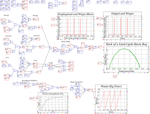
I will work with Tim and Matheus to write this model up for publication in an academic journal over the next few months.
References
Blatt, John M. 1983. Dynamic economic systems: a post-Keynesian approach (Routledge: New York).
Goodwin, Richard M. 1967. ‘A growth cycle.’ in C. H. Feinstein (ed.), Socialism, Capitalism and Economic Growth (Cambridge University Press: Cambridge).
Hicks, J. R. 1935. ‘Wages and Interest: The Dynamic Problem’, The Economic Journal, 45: 456-68.
———. 1937. ‘Mr. Keynes and the “Classics”; A Suggested Interpretation’, Econometrica, 5: 147-59.
Hicks, John. 1981. ‘IS-LM: An Explanation’, Journal of Post Keynesian Economics, 3: 139-54.
Keen, Steve. 2001. Debunking economics: The naked emperor of the social sciences (Pluto Press Australia & Zed Books UK: Annandale Sydney & London UK).
———. 2020. ‘The appallingly bad neoclassical economics of climate change’, Globalizations: 1-29.
Keen, Steve, Timothy Lenton, T. J. Garrett, James W. B. Rae, Brian P. Hanley, and M. Grasselli. 2022. ‘Estimates of economic and environmental damages from tipping points cannot be reconciled with the scientific literature’, Proceedings of the National Academy of Sciences, 119: e2117308119.
Keynes, J. M. 1936. The General Theory of Employment, Interest and Money ( Macmillan: London).
Lorenz, Edward N. 1963. ‘Deterministic Nonperiodic Flow’, Journal of the Atmospheric Sciences, 20: 130-41.
Lucas, Robert E., Jr. 2004. ‘Keynote Address to the 2003 HOPE Conference: My Keynesian Education’, History of political economy, 36: 12-24.
Prescott, Edward C. 1999. ‘Some Observations on the Great Depression’, Federal Reserve Bank of Minneapolis Quarterly Review, 23: 25-31.
Ramsey, F. P. 1928. ‘A Mathematical Theory of Saving’, The Economic Journal, 38: 543-59.