Science-based damage functions for economists

Introduction

Carbon Tracker published Professor Keen’s report Loading the DICE against pensions (Keen 2023) in July 2023. Since then, Carbon Tracker has presented the report to the UK’s Prudential Regulation Authority, who were very supportive. It has been cited in the UK Parliament, and discussed at the EU. The online website Intercept published a very hard-hitting story based on the report on Thursday October 19th 2023. Professor Keen spoke to the report at the European Central Bank on November 7th 2023, and will speak to investors at Jefferies Bank Climate Day on January 24th, 2024.

Carbon Tracker’s report was cited by an Institute and Faculty of Actuaries report entitled The Emperor’s New Climate Scenarios: Limitations and assumptions of commonly used climate-change scenarios in financial services, which was co-authored by the climate scientist Professor Tim Lenton of Exeter University (Trust, Joshi, Lenton, and Oliver 2023). Lenton proposed a way that Keen’s innovation of fitting a logistic damage function to NOAA’s Billion Dollar Damages database could be extended to create a science-based damage function to replace the ones made up by economists. What follows is their joint research proposal. Given the significance of the issue, this project needs funding to enable it to be completed as soon as possible.

Funders of this project thus have an opportunity to be on the right side of history, and as well, could experience a first mover advantage that goes with such a strategy, prior to the release of the refereed academic papers that this research will generate.

The Problem

The economic analysis of climate change has been dominated by damage functions, which map expected levels of global warming to reductions in expected future levels of GWP (Gross World Product). Economists have developed their own empirical methods to calibrate these functions, and this has resulted in the consensus—as shown by a survey of 738 economists who have published in leading economics journals—that a trajectory towards 7°C of warming in 2 century’s time will reduce GWP in 2220 by 20%, compared to what GWP would have been in the absence of global warming (Howard and Sylvan 2021, Figure 11, p. 23).

When estimated damages to future GWP are translated into a rate of annual economic growth, a 20% decline in GWP in 2220 means a fall in the annual rate of economic growth for the next two centuries of a mere 0.02% per annum. This is 1/5th of the accuracy with which economic growth is measured today, which implies that global warming will have imperceptible impact on human welfare, even out to 7°C of warming. This attitude is confirmed by the economics chapter of the IPCC 2014 report, which declared that:

For most economic sectors, the impact of climate change will be small relative to the impacts of other drivers (medium evidence, high agreement). Changes in population, age, income, technology, relative prices, lifestyle, regulation, governance, and many other aspects of socioeconomic development will have an impact on the supply and demand of economic goods and services that is large relative to the impact of climate change. (IPCC et al. 2014, p. 662)

Similarly, the 2022 IPCC report’s economics chapter asserted that “warming of ~4°C may cause a 10–23% decline in annual global GDP by 2100 relative to global GDP without warming”, which implies a fall in the annual rate of economic growth of between 0.1% and 0.3% per annum. This is between a 20th and a 50th of the impact that the Global Financial Crisis had on annual economic growth between 2007 and 2010.

This economic consensus of trivial damages from substantial global warming cannot be reconciled with the scientific literature on climate change, where, for example, Xu and Ramanathan have described 3°C of warming as “catastrophic” and 5°C or more of warming as “implying beyond catastrophic, including existential threats” (Xu and Ramanathan 2017, p. 10315). But policymakers, the media, and most economic consultants are unaware of this “huge gulf between natural scientists’ understanding of climate tipping points and economists’ representations of climate catastrophes” (Lenton and Ciscar 2013, p. 585). Instead, they appear to treat the estimates by economists as if they were simply a translation of the physical dangers expected by scientists into the economic measure of changes to GWP.

This is far from the case. Instead, economists have calibrated their damage functions using approaches that betray a fundamental misunderstanding of what global warming is (Keen 2023, 2020; Trust, Joshi, Lenton, and Oliver 2023; Lenton et al. 2023; Keen et al. 2022). We are very confident that, had the empirical methods used by economists been refereed by scientists, then not one of the 39 key papers from which all “economics of climate change” papers and “Integrated Assessment Models” (IAMs) have been derived (Tol 2022, Table 1, pp. 19-20) would have been published.

Unfortunately, this did not happen, so that trivial and manifestly erroneous estimates of the economic damages from global warming have become the foundation of how the dangers of climate change have been assessed for both policy formation and portfolio allocation.

We cannot turn back time and prevent these papers—or their modelling offspring of IAMs—from being created. We have to accept that climate change policy will be dominated by economic damage functions. But we can produce science-based damage estimates that can displace the deluded estimates made up by economists, so that IAMs will instead generate estimates of damages to GWP that are based on scientific knowledge, rather than economic fantasy.

The Proposal

In his report for Carbon Tracker, Keen showed the impact of extrapolating current climate change damages forward using a logistic function, rather than the quadratic function that is the default in economic IAMs (Keen and Hanley 2023, pp. 37-46; Keen 2023, pp. 36-40). Lenton developed this idea further in The Emperor’s New Climate Scenarios (Trust, Joshi, Lenton, and Oliver 2023), suggesting that:

A practical fix may be to ‘invert’ scenario analysis and use a reverse stress test approach, as used in financial services risk management. This would start with what we want to avoid, then work backwards from there. (Trust, Joshi, Lenton, and Oliver 2023, p. 24)

These ideas have been combined by Keen and Lenton into a method for developing damage functions using the wisdom of scientists, rather than the delusions of economists.

Lenton and Keen will replicate the Howard and Sylvan survey, but with scientists who have published climate change papers in the top 25 science journals. The scientists would be surveyed on the temperature level they believe would lead to the complete collapse of humanity’s agricultural and industrial systems.

A logistic function will be used to back cast from the scientific consensus—which we expect to lie in the range of 3-5°C. A high-order polynomial damage function will be derived from this function, and this would be used in place of the normally quadratic damage functions currently used by economists (this is necessitated by the fact that the programs economists use to simulate economic damages—such as GAMS, in which Nordhaus’s DICE model is estimated—cannot handle logistic functions).

This on its own is not enough however: economists could ignore this function, as they have ignored past criticisms, and they could continue using their own erroneous damage estimates. These papers need to be removed from academic literature. We will do ex-post what should have been done ex-ante: scientists will referee the strictly climate-change aspects of economic papers on economic damages from global warming. If this refereeing process recommends that these papers should not have been published, then we will contact the relevant journals to insist that the publication of these papers be rescinded.

Even if these economic journals so not comply with that request, any consultant or body with fiduciary responsibilities will arguably be in breach of those duties if they continue using damage functions based on the work of economists.

The Team

Professor Keen is a Distinguished Research Fellow at University College London. Professor Lenton holds the Chair in Climate Change at the University of Exeter.

Keen and Lenton are uniquely qualified to undertake this proposal.

Keen has been a long-standing critic of mainstream economics, and is a leading developer of an alternative paradigm—see his popular books Debunking Economics (Keen 2011) and The New Economics: A Manifesto (Keen 2021). He is recognized as one of the 20 most influential economists in the world today by the Academic Influence website (see Top Influential Economists Today | Academic Influence).

There have been many critics of the work by economists on climate change (Ackerman and Munitz 2012; Ackerman and Stanton 2008; Ackerman, Stanton, and Bueno 2010; Aldred 2012; Auffhammer 2018; Auffhammer, Hsiang, Schlenker, and Sobel 2013; Cline 1992; Darwin 1999; DeCanio 2003; Howard and Sterner 2017; Pindyck 2013, 2017; Stern 2022; Stern, Stiglitz, and Taylor 2022). Remarkably however, none of these papers criticised the absurd empirical assumptions that “climate change economists” have made.

This may reflect the mainstream economic attitude that “assumptions don’t matter” (Friedman 1953). However that belief applies, if at all, only to “simplifying assumptions”. In contrast, these manifestly false assumptions are critical to the conclusions by economists that damages from climate change will be slight. Since these assumptions are wrong, so are their conclusions. Keen was the first to criticise these assumptions, originally in “The appallingly bad neoclassical economics of climate change” (Keen 2020), and then in Carbon Tracker’s report (Keen and Hanley 2023; Keen 2023).

Lenton is a climate scientist who has long been aware of the ludicrous assumptions that economists have made to trivialise the dangers of climate change (Lenton and Ciscar 2013). He has also previously conducted a very careful expert survey of climate scientists to assess the likelihood of climate tipping points being triggered (Lenton et al. 2008). He has been a prominent contributor to the academic literature on tipping points, which was recognized by the OECD when he was commissioned to assess the possible impacts of losing the AMOC (OECD 2021).

The Methods

This research project will lead the development of scientifically sound damage function suitable for economists’ Integrated Assessment Models (IAMs), using three methods:

  1. An expert survey, similar in design to (Howard and Sylvan 2021, p. 23), would be used to identify temperature increases that climate change scientists expect would terminate human industrial civilisation. A logistic damage function would then be extrapolated back to current and pre-industrial temperatures from the median and range of such temperature estimates.
  2. An empirical assessment of the temperature increase to GWP relationship will also be undertaken, using wet bulb temperature (WBT) rather than ambient surface temperature. WBT takes into account both temperature and humidity, and provides a more comprehensive understanding of the actual thermal conditions, which are a better indicator of the climatic impact on people’s ability to work and survive. Using WBT offers a more nuanced and insightful approach to understanding the impacts of climate change on various sectors of the economy. This method would provide a physically grounded alternative damage function. It would also enable the survey-based damage function to be applied on a country-by-country basis.
  3. The project will also address the question of the scientific credibility of the estimates that economists have made of economic damages from climate change. There are, according to Tol, a mere 39 papers that are the basis of the empirical estimates that economists have given of damages from climate change (Tol 2022, Table 1, p. 19), along with a similarly small number of studies of the economic impact of triggering tipping points (Dietz, Rising, Stoerk, and Wagner 2021). We contend that had scientists refereed the strictly climate-change and global-warming aspects of these papers, then none of them would have been published. We will test this hypothesis by assembling a panel of climate scientists to ex-post referee these papers.

The Outcomes

  1. Two damage functions will be generated, which should in future be used by economists in IAM studies. These will be a replacement for the damage functions that economists currently use, which are normally quadratic—such as the damage function in Nordhaus’s DICE IAM:

    The parameter used in the model was … 0.227 percent loss in global income per degrees Celsius squared with no linear term. This leads to a damage of 2.0 percent of income at 3°C, and 7.9 percent of global income at a global temperature rise of 6°C. (Nordhaus 2018, p. 345)

    Given the serious problems with the empirical methods used by economists to date, a damage function developed by scientists is virtually certain to generate much higher damage estimates than are made in the existing literature on the economics of global warming.

  2. Papers establishing that the empirical assumptions by economists about climate change are false will be published in leading science journals. These papers will call on economic journals to withdraw all economic papers whose empirical assumptions about global warming are rejected by the panel of scientific referees.
  3. The project leaders, in conjunction with supporting organisations like Carbon Tracker, will contact the editors of the journals which published any of these papers that are rejected in this ex-post refereeing process, to insist that their publication be retracted.

Budget

The project needs to be completed as quickly as possible, given the urgency of the climate crisis, and expectations by some scientists of a 0.5°C increase in temperatures in 2024. We have budgeted to allow the project principals to work on this full-time, and to employ a market research company to manage the practical aspects of the survey.

Component

Expected Cost

Senior Research Fellows (2) salaries plus on-costs

£360,000

Senior Research Impact Fellow

£120,000

Market Research Company Survey Fees

£200,000

Refereeing payments: £750 per paper x 4 referees x 40 papers

£120,000

Preparatory Workshop

£60,000

Postdoctoral Fellow

£85,000

Postdoctoral Associate

£67,000

Administrative Assistant

£50,000

Publicity budget

£200,000

Total

£1,262,000

References

Ackerman, Frank, and Charles Munitz. 2012. ‘Climate damages in the FUND model: A disaggregated analysis’, Ecological Economics, 77: 219-24.

Ackerman, Frank, and Elizabeth A. Stanton. 2008. ‘A comment on “Economy-wide estimates of the implications of climate change: Human health”‘, Ecological Economics, 66: 8-13.

Ackerman, Frank, Elizabeth A. Stanton, and Ramón Bueno. 2010. ‘Fat tails, exponents, extreme uncertainty: Simulating catastrophe in DICE’, Ecological Economics, 69: 1657-65.

Aldred, Jonathan. 2012. ‘Climate change uncertainty, irreversibility and the precautionary principle’, Cambridge Journal of Economics, 36: 1051-72.

Auffhammer, Maximilian. 2018. ‘Quantifying Economic Damages from Climate Change’, Journal of Economic Perspectives, 32: 33-52.

Auffhammer, Maximilian, Solomon M. Hsiang, Wolfram Schlenker, and Adam Sobel. 2013. ‘Using Weather Data and Climate Model Output in Economic Analyses of Climate Change’, REV ENV ECON POLICY, 7: 181-98.

Cline, W.R. 1992. The Economics of Global Warming (Institute for International Economics: Washington, D.C.).

Darwin, Roy. 1999. ‘The Impact of Global Warming on Agriculture: A Ricardian Analysis: Comment’, The American Economic Review, 89: 1049-52.

DeCanio, Stephen J. 2003. Economic models of climate change : a critique (Palgrave Macmillan: New York).

Dietz, Simon, James Rising, Thomas Stoerk, and Gernot Wagner. 2021. ‘Economic impacts of tipping points in the climate system’, Proceedings of the National Academy of Sciences, 118: e2103081118.

Friedman, Milton. 1953. ‘The Methodology of Positive Economics.’ in, Essays in positive economics (University of Chicago Press: Chicago).

Howard, Peter H., and Thomas Sterner. 2017. ‘Few and Not So Far Between: A Meta-analysis of Climate Damage Estimates’, Environmental and Resource Economics, 68: 197-225.

Howard, Peter, and Derek Sylvan. 2021. “Gauging Economic Consensus on Climate Change.” In. New York: Institute for Policy Integrity, New York University School of Law.

IPCC, D.J. Arent, R. S. J. Tol, E. Faust, J.P. Hella, S. Kumar, K.M. Strzepek, F.L. Tóth, and D. Yan. 2014. ‘Key economic sectors and services.’ in C.B. Field, V.R. Barros, D.J. Dokken, K.J. Mach, M.D. Mastrandrea, T.E. Bilir, M. Chatterjee, K.L. Ebi, Y.O. Estrada, R.C. Genova, B. Girma, E.S. Kissel, A.N. Levy, S. MacCracken, P.R. Mastrandrea and L.L. White (eds.), Climate Change 2014: Impacts, Adaptation, and Vulnerability. Part A: Global and Sectoral Aspects. Contribution of Working Group II to the Fifth Assessment Report of the Intergovernmental Panel on Climate Change (Cambridge University Press: Cambridge, United Kingdom).

Keen, S., and Brian P. Hanley. 2023. “Supporting Document to the DICE against pensions: how did we get here?” In. London: Carbon Tracker.

Keen, Steve. 2011. Debunking economics: The naked emperor dethroned? (Zed Books: London).

———. 2020. ‘The appallingly bad neoclassical economics of climate change’, Globalizations: 1-29.

———. 2021. The New Economics: A Manifesto (Polity Press: Cambridge, UK).

———. 2023. “Loading the DICE against pension funds: Flawed economic thinking on climate has put your pension at risk ” In. London: Carbon Tracker.

Keen, Steve, Timothy Lenton, T. J. Garrett, James W. B. Rae, Brian P. Hanley, and M. Grasselli. 2022. ‘Estimates of economic and environmental damages from tipping points cannot be reconciled with the scientific literature’, Proceedings of the National Academy of Sciences, 119: e2117308119.

Lenton, Timothy, and Juan-Carlos Ciscar. 2013. ‘Integrating tipping points into climate impact assessments’, Climatic Change, 117: 585-97.

Lenton, Timothy M., Hermann Held, Elmar Kriegler, Jim W. Hall, Wolfgang Lucht, Stefan Rahmstorf, and Hans Joachim Schellnhuber. 2008. ‘Tipping elements in the Earth’s climate system’, Proceedings of the National Academy of Sciences, 105: 1786-93.

Lenton, Timothy M., Chi Xu, Jesse F. Abrams, Ashish Ghadiali, Sina Loriani, Boris Sakschewski, Caroline Zimm, Kristie L. Ebi, Robert R. Dunn, Jens-Christian Svenning, and Marten Scheffer. 2023. ‘Quantifying the human cost of global warming’, Nature Sustainability.

Nordhaus, William. 2018. ‘Projections and Uncertainties about Climate Change in an Era of Minimal Climate Policies’, American Economic Journal: Economic Policy, 10: 333–60.

OECD. 2021. Managing Climate Risks, Facing up to Losses and Damages.

Pindyck, Robert S. 2013. ‘Climate Change Policy: What Do the Models Tell Us?’, Journal of Economic Literature, 51: 860-72.

———. 2017. ‘The Use and Misuse of Models for Climate Policy’, Review of Environmental Economics and Policy, 11: 100-14.

Stern, Nicholas. 2022. ‘A Time for Action on Climate Change and a Time for Change in Economics’, The Economic Journal, 132: 1259-89.

Stern, Nicholas, Joseph Stiglitz, and Charlotte Taylor. 2022. ‘The economics of immense risk, urgent action and radical change: towards new approaches to the economics of climate change’, Journal of Economic Methodology, 29: 181-216.

Tol, R. S. J. 2022. “A meta-analysis of the total economic impact of climate change.” In.: arXiv.org.

Trust, Sandy, Sanjay Joshi, Timothy Lenton, and Jack Oliver. 2023. “The Emperor’s New Climate Scenarios: Limitations and assumptions of commonly used climate-change scenarios in financial services.” In. London: Institute and Faculty of Actuaries.

Xu, Y., and V. Ramanathan. 2017. ‘Well below 2 °C: Mitigation strategies for avoiding dangerous to catastrophic climate changes’, Proceedings of the National Academy of Sciences of the United States of America, 114: 10315-23.


Using system dynamics with Minsky to prove the core tenets of MMT

Abstract

Modern Monetary Theory (MMT) is a non-mainstream economic theory that contradicts conventional economic analysis of government debt and deficits. We use the system dynamics program Minsky to develop a mathematical model of MMT. This model shows that the core tenets of MMT are correct, and Neoclassical arguments about government debt and deficits are wrong.

Introduction

A common criticism of MMT by Neoclassical economists is that it lacks a mathematical framework:

MMT theorists have never subjected their theory to formal treatment by mathematical modeling (Bossone 2021, p. 162).

MMT lacks theoretical analysis based on mathematical models compared to mainstream economics, which is based on a neoclassical framework. (Tanaka 2021, p. 2)

These critics then proceed to examine MMT using the tools of Neoclassical economic theory:

the choice of using ISLM analysis for the purpose of this article is not driven by which model should best describe the economy in general, but rather by which model can best mirror the economic relations underpinning MMT, in the absence of a formal representation by its proponents, while subjecting them to consistency checks. (Bossone 2021, p. 163. Emphasis added)

In this paper, we try to argue positively for the idea of the effect of fiscal policy, which is the backbone of functional finance theory and MMT’s argument, using a simple mathematical model, while maintaining the basics of the neoclassical microeconomic framework, such as utility maximization of consumers by utility function and budget constraint [sic.], profit maximization of firms in monopolistic competition, and equilibrium of supply and demand of goods. (Tanaka 2021, p. 2. Emphasis added)

A common retort by MMT economists is that Neoclassical models of money are simply wrong. Kelton observes that:

MMT rejects the loanable funds story, which is rooted in the idea that borrowing is limited by access to scarce financial resources. As MMT economist Scott Fullwiler put it, the conventional “analysis is simply inconsistent with how the modern financial system actually works.” (Kelton 2020, p. 113)

If the conflict between these two paradigms is to be resolved, we need a mathematical framework which is consistent with how the modern financial system actually works. The Open-Source system dynamics program Minsky provides that framework.

Minsky, the software

Minsky is named in honour of the great Post-Keynesian economist Hyman Minsky (Minsky 1982), who developed the “Financial Instability Hypothesis” (Minsky 1977) as a realistic alternative to the Neoclassical “Efficient Markets Hypothesis”, which underlies the “Capital Asset Pricing Model” (Fama and French 2004; Sharpe 1964). Minsky supports the standard system dynamics tools of flowchart modelling,
and in addition
provides Godley Tables—named after another great Post-Keynesian, Wynne Godley (Godley 1999)—which enable easy modelling of financial stock and flows.

A Godley Table records financial transactions following the principles of double-entry bookkeeping (Gleeson-White 2011), that:

  • All financial claims are classified as either Assets or Liabilities;
  • One entity’s financial Asset is another entity’s financial Liability; and
  • All transactions are recorded twice, subject to the fundamental rule of accounting that Assets (A) minus Liabilities (L) equals Equity (E).

The entries in a Godley Table generate a set of differential equations describing the model of the financial system. So long as every transaction is properly recorded, then the model is structurally correct.

Figure 1 shows a blank Godley Table.

Figure 1: A blank Godley Table (as seen in the Edit window)

Stocks (financial assets and liabilities) are defined on the row beginning “Flows¯/Stock Vars®” in Figure 1, and are added, deleted and moved using the +,- and ¬® buttons. Flows (financial transactions) are defined on the rows of the Table, with two entries required per row. These entries must obey the rule that , which is checked by the final column in the table. Minsky uses the rule that one entity’s asset is another’s liability to enable an integrated model of the financial system to be developed. The wedge symbol q accesses a drop-down menu showing Assets that have not yet been recorded as Liabilities for another entity, and vice versa.

A quick primer on Minsky

Figure 2 shows a simple economic model, in which bank lending creates both Loans and Deposits. Borrowers then pay interest, and the banks purchase goods and services from the non-bank private sector.

Figure 2: A simple model of bank-originated money and debt


The Godley Tables generate the differential equations of the model, since the symbolic sum of a column is the rate of change of the relevant stock:


The flows are defined on the design canvas using mathematical operators. Variables and parameters can be copied and used in multiple locations on the canvas if desired. Parameter values can be altered during a simulation, using either arrow keys or the “dot” slider on top of the parameter.

Minsky generates the equations for the model, which can be exported in LaTeX format for documentation purposes—see Equation (1) and (2).


This model could easily be developed in any system dynamics program using flowchart logic, but there is an enormous advantage in using Godley Tables instead. The entire financial system operates on the principles of double-entry bookkeeping, which has the same status In the analysis of monetary systems as the Laws of Thermodynamics have in the analysis of energy. We therefore paraphrase Sir Arthur Eddington’s marvellous put-down of models in physics that violate the Second Law of Thermodynamics (Eddington 1928, p. 37):

The rules of double-entry bookkeeping hold the supreme position among the laws of Money. If your theory is found to be against the rules of double-entry bookkeeping, we can give you no hope; there is nothing for it but to collapse in deepest humiliation.

Minsky‘s Godley Tables ensure that these rules are obeyed, and it therefore acts not only as an enabler of accurate financial modelling, but also as a prohibition: actions which might be possible to model in standard flowchart notation can violate double-entry bookkeeping, and are therefore wrong.

A clear example here is the model of “Fractional Reserve Banking”, which gives rise to the “Money Multiplier” theory of money creation, and which is taught by all conventional economic textbooks. This is an extract from the popular textbook Principles of Macroeconomics by Mankiw:

Deposits that banks have received but have not loaned out are called reserves… After the bank opens and people deposit their currency, the money supply is the $100 of demand deposits… Let’s suppose that First National has a reserve ratio of … 10 percent … it keeps 10 percent of its deposits in reserve and loans out the rest… It turns out that even though this process of money creation can continue forever, it does not create an infinite amount of money. If you laboriously add the infinite sequence of numbers in the preceding example, you find the $100 of reserves generates $1,000 of money. (Mankiw 2016, pp. 332-334)

This model is also clearly believed by economic policymakers. This is how then Federal Reserve Chairman Ben Bernanke explained why Quantitative Easing was being undertaken in the aftermath to the Global Financial Crisis:

Large increases in bank reserves brought about through central bank loans or purchases of securities are a characteristic feature of the unconventional policy approach known as quantitative easing. The idea behind quantitative easing is to provide banks with substantial excess liquidity in the hope that they will choose to use some part of that liquidity to make loans or buy other assets. (Bernanke 2009, p. 5. Emphasis added)

This process of “lending out Reserves” is easily modelled using the flowchart method: see Figure 3.

Figure 3: The “Money Multiplier” portrayed in a conventional system dynamics format

However, when this model is laid out using a Godley Table, there is an obvious problem: directly “lending from Reserves” violates double-entry bookkeeping: see Figure 4.


Figure 4: Lending directly from Reserves violates the fundamental rules of accounting

Figure 4 is doubly wrong because it also doesn’t create any loans. The only way to show Loans being created is to have Reserves fall and Loans rise by the same amount, as in Figure 5.

Figure 5: No violation of accounting, but how do borrowers get the money?

This now accords with the rules of accounting, but at this stage there is an additional liability for borrowers (increased Loans) but no additional assets (increased money). To show borrowers getting money from the loans, we have to include the Private Sector’s Godley Table, and show that some other Private Sector asset rises to compensate for this increase in the Private Sector’s liabilities. This asset is Cash: the borrowers’ cash holdings rise by the amount of the loans, and the borrowers then re-deposit this cash at the banks—see Figure 6.

Figure 6: The Money Multiplier only works if the entire monetary system operates with cash

The simple model now works as a way to create money, but only under two absurd conditions: not only must all loans be in cash, the entire monetary system—including Reserves—must be cash-based. You can get rid of needing Reserves to be cash-based by a much more complicated model, but you cannot escape the requirement that loans themselves must be in cash.

This is fallacious as a description of modern banking. While it may have been approximately the case in the 19th century, it is ridiculous today, when the vast majority of loans are electronic.

Mainstream economic models of money—both the “Money Multiplier” and “Loanable Funds”—face humiliation when expressed in terms of double-entry bookkeeping. The core tenets of MMT, on the other hand, are derived from the principles of double-entry bookkeeping.

MMT

The Government Deficit is the Private Surplus

Figure 7 shows the essential government operations of spending and taxation as seen from the point of view of the Banking Sector.

Figure 7: Government spending and taxation shown on the Banking Sector’s Godley Table

As with the private money creation dynamics outlined in Figure 2, these entries cascade through the financial accounts of the other sectors—shown via Godley Tables in Minsky. Reserves are a Liability of the Central Bank, while Bonds are a Liability of the Treasury. Figure 8 shows the consequences of laying out the transactions in Figure 7 for the other sectors, and this shows that the model is incomplete: there is as yet no account against which to record the second double-entry for both spending and taxation on the Central Bank’s table.

Figure 8: The basic but incomplete view of government spending and taxation


This indicates that there is another account which must be added to the model: the Treasury’s account at the Central Bank. This is commonly known as the Consolidated Revenue Fund (CRF), and we call it TreasuryCRF here. Figure 9 shows this completed fundamental model.

Figure 9: The basic complete view of government spending and taxation

Figure 9, and the equations of this model in Equation , confirm the core MMT insight that the government deficit IS the private sector surplus. If government spending exceeds taxation, then the private sector’s net financial worth—its equity—rises by , which is precisely the sum by which the government sector’s net financial worth falls. This is obvious in the non-zero differential equations which Minsky generates from the tables in Figure 9:


The MMT ab-initio argument first made by Warren Mosler (Mosler 2010), that the government must spend before it can tax, is also confirmed by these equations. For fiat money to exist, the government must first spend it into existence.

This explains the fundamental nature of fiat money. Fiat money is created by a government issuing net financial liabilities upon itself, which in turn creates net financial assets for the non-government sector.

If the government does not spend more than it takes back in taxation, then it does not create fiat money—and a surplus actually destroys fiat money. Mainstream economists who object to the government running a deficit are in fact objecting to the creation of fiat money.

Fiat money gives the non-government sector a means to undertake monetary transactions by exchanging the government’s liabilities—fiat money—with each other. Without fiat money, the only liabilities that can be exchanged are those created by the banking sector: credit money. Fiat money creation also increases the net financial worth of the non-government sector, whereas credit-based money does not.

Finally, both credit and fiat money creation work by increasing the Assets of the Banking Sector simultaneously with increasing the Liabilities. Credit money creation increases Loans, which are an income earning asset for the Banking Sector. Fiat money creation increases Reserves, which—prior to the Global Financial Crisis (GFC)—were not an income-earning asset for the Banking Sector.

A Conservation Law

Minsky reveals a fundamental but thus far overlooked aspect of a monetary economy: the conservation law that the sum of all financial equities is zero. Since every entity’s financial asset is another entity’s financial liability, in the aggregate, the net financial equity of every sector identically equals the negative of the net financial equity of all other sectors. This mathematical truism provides a reason to support fiat money—and hence government deficits—that even Austrian economists might be able to comprehend: without government deficits, the non-bank private sector is necessarily in negative financial equity.

A bank must have positive net worth: its short-term assets must exceed its short-term liabilities, otherwise it is bankrupt. Therefore, in the absence of a government sector, the non-bank private sector must be in negative equity: its financial liabilities must exceed its financial assets. However, with a government sector that is in sufficient negative equity, it is possible for both the private banking sector and the non-bank private sector to be in positive financial equity.

There has never been an economy without a government, of course, but America in the 19th century and up until WWII provides an example of an economy with a very small government sector (relative to GDP) compared to the post-WWII economy. On several occasions, the government succeeded—for want of a better word—in reducing its debt to zero. This achievement—driven by the same misplaced abhorrence of government negative equity that lies behind today’s politicians desire to reduce government debt—necessarily drove the private non-bank sectors into negative equity. This may well be a factor in the many financial crises that afflicted the US economy up until the start of WWII.

Treasury Bond Sales

Technically speaking, Figure 9 and Equations (2) and describe the only essential operations in fiat money creation. However, governments have imposed additional requirements upon the operations of the Treasury and Central Banks via laws that require the CRF to not be in overdraft, and which prevent the Central Bank from buying bonds directly from the Treasury. We therefore have to introduce Treasury Bond sales in Primary Auctions, and Central Bank purchases of bonds on the Secondary Market.

Treasury bond sales to the banking sector are shown as the flow BondSaleTàB in Figure 10. These are purchased by the banking sector using its Reserves—and these Reserves are created in the first instance by the government deficit.

This confirms the key MMT insight that the funds banks use to buy government bonds are created by the deficit itself. The purchase of the bonds neither creates money, nor takes money from the private sector, since both transactions occur only on the Asset side of the Banking Sector’s ledger. Treasury Bond sales to the Banking Sector are an asset swap for the banks: they do not constitute borrowing (though they do initiate interest payments, which we consider next). Exchanging Reserve funds for Bonds enables banks to part with a non-tradeable asset (and until the GFC, non-income-earning asset) which was created by the Treasury, for a tradeable, income-earning asset which was also created by the Treasury.

Figure 10: Sales of Treasury Bonds to the Banking Sector

The main practical impact of this transaction is on the Treasury’s account at the Central Bank. If the government habitually runs a deficit, then its account at the Central Bank will have more outflows than inflows, and will necessarily turn negative. Almost all governments have passed laws requiring their Treasuries not to be in overdraft to the Central Bank, and this is what Bond sales achieve: if Bond sales are equal to the deficit, then the Treasury’s Consolidated Revenue Fund (CRF) at the Central Bank can remain non-negative—see Figure 11.

Figure 11: The government sector view of Treasury Bond sales

Interest on Treasury Bonds

Introducing bond sales made no difference to government money creation. Interest on bonds, on the other hand, does. Figure 12 shows that interest on bonds owned by Banks adds to the net worth of the Banking Sector.

Figure 12: Interest on Bonds from the Banking Sector’s Perspective

This necessarily increases the negative net financial worth of the government sector. The rate of change of the Treasury’s equity now equals —see Figure 13. Maintaining a non-zero balance in the Treasury’s CRF requires the Treasury to issue bonds equivalent to the deficit plus interest on outstanding bonds held by the non-government sector.

Figure 13: Interest on Bonds from the Government’s Perspective

Central Bank Open Market Operations

A notable feature of the model thus far is that the Central Bank has no assets. This is addressed by considering Central Bank Open Market Operations (OMO). Though these are undertaken primarily to keep the interest rate on bonds within the Central Bank’s target range, the effect of net Bond purchases by the Central Bank is to create positive assets it. If, hypothetically, these net purchases equal the interest paid on bonds owned by the Government sector, then the potential for the exponential growth of government “debt” (in reality, of Treasury bonds owned by the non-Government sector), which has led to some internet chatter in recent months, will not be realised, since around the globe, Treasuries either do not pay interest on bonds owned by other sectors of the government, or Central Banks remit their earnings to the Treasury.

Figure 14: Open Market Operations by the Central Bank

Bank Sales of Bonds to Non-Banks

The final detail needed to portray the basic operations of fiat money creation is the sale of bonds by banks to the non-bank private sector—and primarily to Non-Bank Financial Institutions (NBFIs). This is one of the only two bond operations which change the amount of money in the economy—the other being Open Market Operations (including “Quantitative Easing” and “Quantitative Tightening”) with NBFIs. Bonds sales by Banks to NBFIs are executed by debiting the deposit accounts of NBFIs at the Banks, which reduces the money supply.

These operations complete the basic double-entry-based view of the operations involved in fiat money creation. The full structure is shown in Figure 15.

Figure 15: The complete structural model of fiat money operations

The non-zero differential equations of this process are shown in Equation :


A Summing Up

The main characteristics of this systemic description of government finances, derived directly from double-entry bookkeeping, are:

  • Government spending in excess of taxation is financed by the government going into negative financial equity to the same magnitude, which creates equivalent positive financial equity for the non-government sectors. The condition under which the government creates positive financial equity for the non-government sector is:


  • In this simple model, the money supply is the sum of Deposits and the banking sector’s short-term equity BanksE. The operation in Equation creates money for the non-government sectors, so long as this positive equity is greater than bond sales to non-banks by the private banks and Central Bank:


  • Bond sales by the Treasury are undertaken to maintain a non-negative balance for the Treasury’s Consolidated Revenue Fund at the Central Bank. This condition will hold so long as:


  • The funds used by the banking sector to buy government bonds are created by the government Deficit—the excess of government spending and interest payments over taxation—which increases the Banking Sector’s Reserves; the money used by the non-bank private sector to buy bonds is created the same way, since the Deficit also creates Deposits; and
  • Interest on government bonds is a fiat-money-financed source of income for the private sector.

These deductions are all consistent with the basic tenets of MMT, as set out in The Deficit Myth (Kelton 2020). In contrast, the attitudes of Neoclassical economics towards budget deficits are inconsistent with double-entry bookkeeping.

The Neoclassical Approach to Budget Deficits

Mankiw’s textbook Principles of Macroeconomics (Mankiw 2016) is typical of the Neoclassical treatment of government deficits. Mankiw situates his analysis within the model of Loanable Funds:

To keep things simple, we assume that the economy has only one financial market, called the market for loanable funds. All savers go to this market to deposit their saving, and all borrowers go to this market to take out their loans. Thus, the term loanable funds refers to all income that people have chosen to save and lend out, rather than use for their own consumption, and to the amount that investors have chosen to borrow to fund new investment project (Mankiw 2016, p. 268)

Supply and demand analysis, and not double-entry bookkeeping, is thus the foundation of the Neoclassical critique of MMT. The correct domain of supply and demand analysis is the production and consumption of goods and services, and even there it has enormous problems (Keen 2024; Keen 2021, 2011). Here, supply and demand analysis in the form of Loanable Funds ignores double-entry bookkeeping, and does not explain the creation of money: instead, it takes the money supply as given, and discusses its allocation, in that any money that is not spent on consumption is assumed to be the source of loanable funds:

The supply of loanable funds comes from people who have some extra income they want to save and lend out… saving is the source of the supply of loanable funds. (Mankiw 2016, p. 268)

One of several fallacies in this analysis is the lumping together of public and private savings, as if they are independent activities:

When the government runs a budget deficit, public saving is negative, and this reduces national saving. In other words, when the government borrows to finance its budget deficit, it reduces the supply of loanable funds available to finance investment by households and firms. (Mankiw 2016, p. 273)

This is easily shown to be false using the Equity Equations in Equation (4). Savings can be defined as the change in equity of an entity, and private saving is the sum of the change in equity of the non-government private sectors (bank and non-banks). This is identically equal to the negative of the change in equity for the government sectors (Central Bank and Treasury). The correct equation is:


Mankiw’s first sentence is thus 100% wrong. The correct statement of the relation between the budget deficit and private savings is:

When the government runs a budget deficit, public saving is negative, and this creates private savings. In other words, when the government runs a deficit, it increases the supply of bank deposits available to finance consumption and investment by households and firms.

Mankiw also asserts that a government deficit decreases the supply of funds available for private investment:

Thus, the most basic lesson about budget deficits follows directly from their effects on the supply and demand for loanable funds … the government reduces national saving by running a budget deficit … The model as presented here takes this term [Loanable Funds] to mean the flow of resources available to fund private investment; thus, a government budget deficit reduces the supply of loanable funds… a budget deficit increases the interest rate, thereby crowding out private borrowers who are relying
on financial markets to fund private investment projects. (Mankiw 2016, p. 274. Emphasis added)

These deductions are the exact opposite of the real impact of government deficits. The deficit increases the money supply, and therefore the money available to the private sector for both investment and consumption expenditures. This is likely to reduce the demand for credit-based money, which if anything will reduce commercial interest rates, and/or increase the level of investment.

Disentangling Cause and Effect with Minsky

Advocates of austerity often point to the prosperity of years in which America ran surpluses and reduced government debt—specifically the Coolidge and Clinton Presidencies. Predictably—given the mainstream attitude that lending is a “pure redistribution” which should have “no significant macroeconomic effects” (Bernanke 2000, p. 24)—they ignore what happened to private debt at the same time. As federal debt fell from 27% of GDP in 1920 to 16% in 1929, private debt rose from 121% to 156%: see Figure 16.

Figure 16: Debt, Deficits and Credit from 1916-1976

Thus, as the Coolidge administration ran a surplus of 1% of GDP, private sector credit grew at an average of 8% of GDP per year—see Figure 17.

Figure 17: The Deficit, Credit and Growth 1921-28

Minsky enables us to untangle these two factors to see what really caused the growth of the 1920s, by creating a model with both credit and fiat money creation—see Figure 18:

Figure 18: A simple mixed fiat and credit model in Minsky


Reproducing the average rates of credit growth and fiat money contraction in the 1920s caused by Coolidge’s surpluses reproduces much the same economic outcomes: a high rate of economic growth, a falling government debt ratio, and a rising private debt ratio—see Figure 19.

Figure 19: A 1% of GDP surplus and 8% of GDP credit growth reproduces the 1920s data

However, the counterfactual of a 1% of GDP surplus with no credit growth produces an entirely different outcome: the one that MMT predicts of a declining GDP—see Figure 20.

Figure 20: Coolidge’s surplus on its own reduces economic growth


Other Aspects of Minsky for system dynamics experts

This paper focuses upon Minsky‘s capabilities in the topic area which inspired its creation, but there are also aspects of Minsky which should be of interest to practitioners of system dynamics in general.

Firstly, Minsky is one of the few system dynamics programs which are both Open Source and free. You can download it from https://sourceforge.net/projects/minsky/.

Secondly, Minsky‘s design philosophy emphasizes transparency: relationships between stocks and flows are explicitly modelled on the canvas, rather than inside text boxes as in the majority of system dynamics programs. Minsky passes values “by name” as well as “by wire”, so the spaghetti diagrams of conventional programs are replaced by much smaller “spiders’ webs” which define parts of a model. This makes it easier to explain a model to a non-specialist.

Thirdly, since it is programmed by a high-performance-computing expert with a PhD in physics, Dr Russell Standish, Minsky is much more “math-centric” than conventional system dynamics programs. It supports tensor mathematics, produces the equations of its models in LaTeX, and provides symbolic rather than simply numerical differentiation.

Minsky also lacks some tools that professional system dynamics modelers rely upon—such as methods to identify loop dominance. We hope to add such features over time, and financial support via Minsky‘s Patreon page https://www.patreon.com/hpcoder/ will help enable this.

However, we realise that voluntary support alone is unlikely to provide sufficient development funds, while system dynamics is still too “esoteric” a field for most system dynamics programs to be commercially viable.

We have therefore developed a commercial extension of Minsky called Ravel, which is targeted at the spreadsheet, Pivot Table, and “Business Intelligence” marketplace. Ravel uses a novel and patented tool for manipulating multidimensional data visually—see Figure 21. We hope that sales revenue from Ravel will enable us to continue developing Minsky for the system dynamics community. Ravel should be available from mid-2024, and will initially be marketed via Patreon.

Figure 21: Ravel uses Minsky’s interface and the Ravel© object to analyse multidimensional data


Why are mainstream models of money so bad?

Mainstream models of money are fallacious, and rely upon obviously false assumptions—that all loans are in cash (the Money Multiplier) or that bank deposits aren’t demand deposits, and that loans aren’t bank assets (Loanable Funds).

It is therefore not MMT that fails the test of mathematical analysis, but mainstream macroeconomics, with its obsession with equilibrium, and its wilful ignorance of the monetary system. But there is little chance of using system dynamics to persuade mainstream economics to abandon its fallacious models of money and adopt realistic ones, because that would result in the rapid unwinding of the entire Neoclassical paradigm.

The core reason that Neoclassical models of the monetary system are so infantile is that their core paradigm ignores money, and treats capitalism as a barter system. Their models of money are therefore not attempts to describe the monetary system, but attempts to justify ignoring the monetary system in macroeconomic modelling.

Their treatment of groundbreaking papers by Central Banks on money creation is indicative here. In 2014, the Bank of England published “Money creation in the modern economy” (McLeay, Radia, and Thomas 2014), which bluntly rejected mainstream models of money creation and endorsed the non-mainstream “Post-Keynesian” models:

Money creation in practice differs from some popular misconceptions — banks do not act simply as intermediaries, lending out deposits that savers place with them, and nor do they ‘multiply up’ central bank money to create new loans and deposits. (McLeay, Radia, and Thomas 2014, p. 14)

This paper—and a similar one from the Bundesbank (Deutsche Bundesbank 2017)—was largely ignored by mainstream economists, while one of the few papers that engaged with it argued that “loanable funds” was preferable to “the money-creation approach” via a bizarre version of “Occam’s Razor”:

We establish a benchmark result for the relationship between the loanable-funds and the money-creation approach to banking. In particular, we show that both processes yield the same allocations when there is no uncertainty. In such cases, using the much simpler loanable-funds approach as a shortcut does not imply any loss of generality. (Faure and Gersbach 2017, p. 107. Emphasis added)

Only Neoclassical economists could combine the words “when there is no uncertainty” with “does not imply any loss of generality” in the one paragraph.

Conclusion

Forrester’s motivation for developing system dynamics can arguably be traced back to his justified incredulity at the state of mathematical modelling in economics in the 1950s. In the note “Dynamic models of economic systems and industrial organizations: Note to the Faculty research seminar. From Jay W. Forrester. November 5, 1956” (Forrester 2003), he made the following observations:

One of the striking shortcomings of most economic models is their failure to reflect adequately the structural form of the regenerative loops that make up our economic system…

Present models neglect to interrelate adequately the flows of goods, money, information, and labor…

Linear equations have usually been used to describe a system whose essential characteristic, I believe, arise from its non-linearities…

Models, suitable only for long-range prediction, are often used with short-term influences and fluctuations omitted. This is justifiable only if the system is sufficiently linear to permit superposition, an assumption which has not been justified or defended and which is probable untrue…

Time intervals of model solutions are often too widely spaced for the predictions being attempted…

Very often the model and its results are judged by the logic with which the model is developed out of its founding assumptions, whereas the failures probably lie in those assumptions. (Forrester 2003, pp. 332-336)

These criticisms remain valid today, while the economics discipline greeted the first large-scale system dynamics model (Forrester 1971) with both hostility and ignorance (Forrester, Gilbert, and Nathaniel 1974; Nordhaus 1973). The dominant paradigm, Neoclassical economics, remains implacably opposed to methods that do not enforce equilibrium as an outcome of a model (Lazear 2000; Blanchard 2018).

The only hope for getting economists to use system dynamics in place of its current reliance upon either algebraic or discrete-time modelling tools is to partner with economists who are dedicated to realism rather than ideology. These economists self-describe themselves as either Post-Keynesian or Modern Monetary Theorists, or both. However, these groups are often unfamiliar with the methods of system dynamics, and use technologies—such as discrete-time modelling (Lavoie and Zezza 2020)—out of the habits of their training, rather than knowledge of the most appropriate tools.

Minsky is the only tool which enables system dynamic modelling in economics, while enforcing a correct analysis of financial flows. We encourage the system dynamics community to become familiar with Minsky, and to support the subcultures within economics that wish to embrace the realism of dynamics, rather than the fantasy of equilibrium.

Appendix

Figure 22: The Money Multiplier Model with electronic reserves

References

Bernanke, Ben. 2009. “The Federal Reserve’s Balance Sheet: An Update.” In Federal Reserve Board Conference on Key Developments in Monetary Policy. Washington, DC: Board of Governors of the Federal Reserve System.

Bernanke, Ben S. 2000. Essays on the Great Depression (Princeton University Press: Princeton).

Blanchard, Olivier. 2018. ‘On the future of macroeconomic models’, Oxford Review of Economic Policy, 34: 43-54.

Bossone, Biagio. 2021. ‘Why MMT can’t work’, International Journal of Economic Policy Studies, 15: 157-81.

Carter, Susan B. 2006. Historical statistics of the United States : earliest times to the present / editors in chief, Susan B. Carter … [et al.] (Cambridge University Press: New York).

Deutsche Bundesbank. 2017. ‘The role of banks, non- banks and the central bank in the money creation process’, Deutsche Bundesbank Monthly Report, April 2017: 13-33.

Eddington, Arthur Stanley. 1928. The Nature Of The Physical World (Cambridge University Press: Cambridge).

Fama, Eugene F., and Kenneth R. French. 2004. ‘The Capital Asset Pricing Model: Theory and Evidence’, The Journal of Economic Perspectives, 18: 25-46.

Faure, Salomon A., and Hans Gersbach. 2017. “Loanable funds vs money creation in banking: A benchmark result.” In CFS Working Paper Series. Frankfurt: Center for Financial Studies (CFS), Goethe University.

Forrester, Jay W. 1971. World Dynamics (Wright-Allen Press: Cambridge, MA).

———. 2003. ‘Dynamic models of economic systems and industrial organizations: Note to the Faculty research seminar. From Jay W. Forrester. November 5, 1956’, System Dynamics Review, 19: 329-45.

Forrester, Jay W., W. Low Gilbert, and J. Mass Nathaniel. 1974. ‘The Debate on “World Dynamics”: A Response to Nordhaus’, Policy Sciences, 5: 169-90.

Gleeson-White, Jane. 2011. Double Entry (Allen and Unwin: Sydney).

Godley, Wynne. 1999. ‘Money and Credit in a Keynesian Model of Income Determination’, Cambridge Journal of Economics, 23: 393-411.

Keen, S. 2024. “Rebuilding Economics from the Top Down.” In. Budapest: Budapest Centre for Long-Term Sustainability & Pallas Athene Publishing House.

Keen, Steve. 2011. Debunking economics: The naked emperor dethroned? (Zed Books: London).

———. 2021. The New Economics: A Manifesto (Polity Press: Cambridge, UK).

Kelton, Stephanie. 2020. The Deficit Myth: Modern Monetary Theory and the Birth of the People’s Economy (PublicAffairs: New York).

Lavoie, Marc, and Gennaro Zezza. 2020. ‘A Simple Stock-Flow Consistent Model with Short-Term and Long-Term Debt: A Comment on Claudio Sardoni’, Review of Political Economy, 32: 459-73.

Lazear, Edward P. 2000. ‘Economic Imperialism’, Quarterly Journal of Economics, 115: 99-146.

Mankiw, N. Gregory. 2016. Principles of Macroeconomics, 9th edition (Macmillan: New York).

McLeay, Michael, Amar Radia, and Ryland Thomas. 2014. ‘Money creation in the modern economy’, Bank of England Quarterly Bulletin, 2014 Q1: 14-27.

Minsky, Hyman P. 1977. ‘The Financial Instability Hypothesis: An Interpretation of Keynes and an Alternative to ‘Standard’ Theory’, Nebraska Journal of Economics and Business, 16: 5-16.

———. 1982. Can “it” happen again? : essays on instability and finance (M.E. Sharpe: Armonk, N.Y.).

Mosler, Warren. 2010. “The Seven Deadly Innocent Frauds.” In.: Valance Co., Inc.

Nordhaus, William D. 1973. ‘World Dynamics: Measurement Without Data’, The Economic Journal, 83: 1156-83.

Sharpe, William F. 1964. ‘Capital Asset Prices: A Theory of Market Equilibrium under Conditions of Risk’, The Journal of Finance, 19: 425-42.

Tanaka, Yasuhito. 2021. ‘An Elementary Mathematical Model for MMT (Modern Monetary Theory)’, Research in Applied Economics.


It’s a Mixed Credit-Fiat World

In contrast to its attitude to private debt, which it ignores, mainstream economics obsesses about government debt. But this volte-face doesn’t besmirch its record of being 100% wrong.

Government debt, mainstream economics tells us, is a scourge to be minimized, if it can’t be entirely avoided. These quotes are from Mankiw’s influential macroeconomics textbook (Mankiw 2016), with indicative passages highlighted:

When a government spends more than it collects in taxes, it has a budget deficit, which it finances by borrowing from the private sector or from foreign governments. The accumulation of past borrowing is the government debt… (555)

The government debt expressed as a percentage of GDP roughly doubled from 25 percent in 1980 to 47 percent in 1995. The United States had never before experienced such a large increase in government debt during a period of peace and prosperity. Many economists have criticized this increase in government debt as imposing an unjustifiable burden on future generations… (557)

These trends led to a significant event in August 2011: Standard & Poor‘s, a major private agency that evaluates the safety of bonds, reduced its credit rating on U.S. government debt to one notch below the top AAA grade. For many years, U.S. government debt was considered the safest around. That is, buyers of these bonds could be completely confident that they would be repaid in full when the bond matured. Standard & Poor’s, however, was sufficiently concerned about recent fiscal policy that it raised the possibility that the U.S. government might someday default. (559)

Increases in government debt are a concern because they place a burden on future generations of taxpayers and call into question the government’s own solvency. (595)

This attitude towards government debt and deficits—that government debt should be minimised, that deficits are undesirable, that interest payments on government debt are a punitive impost on future generations, and that high debt and high interest payments can even lead to a government going bankrupt—are key facets of contemporary politics. They were behind the attempt by the UK Cameron government to run surpluses rather than deficits, on the principle that, by “saving for a rainy day”,60F the government would have more money on hand when crises struck in the future. They lie behind the recurring “debt ceiling” debates in the US Congress. They are the basis of the Eurozone rules, enshrined in the Maastricht Treaty, that government debt should not exceed 60% of GDP, and deficits should be no more than 3% of GDP.

And they are all completely wrong, as is easily shown by looking at the accounting of the mixed credit-fiat monetary system in which we live. I will explain this very, very slowly. It may be tedious to read—it was tedious to write!—but this is necessary, given that utterly fallacious beliefs about the financial system are ingrained into, and damage, our political and social systems, thanks to erroneous mainstream economic thinking.

  1. The Fundamentals of Fiat Money Creation

Figure 37 shows the absolute basic accounting for a Credit money system: banks create money by marking up both sides of their balance sheets. They add Credit dollars per year to Deposits, which are their Liabilities; and they add precisely the same sum to Loans, which are their Assets.

For the non-bank private sector, the act of borrowing also increases its Assets and Liabilities equally: Deposits, which are its Assets, rise by Credit dollars per year, and Loans, which are its Liabilities, rise by precisely the same amount. There is therefore no change in the net worth of either the Banking Sector, or the Non-Bank Private Sector from the creation of credit-money.

Figure 37: The fundamental accounting for Credit Money

The Government’s role in money creation can be considered the same way, by modelling the two fundamental actions of governments: spending on the non-government private sector (either in the form of purchases or transfers), and taxation of the private sector.61F Figure 38 adds these to the Non-Bank Private Sector’s Godley Table in Figure 30, but without completing the double-entry.62F

Figure 38: Introducing Government Spending and Taxation without completing the double-entry

How should it be completed? I hope that it is obvious that the only way to complete this double-entry picture is that government spending increases the Equity—the net financial worth—of the non-bank private sector, while taxation reduces it.

This is shown in Figure 39. Government spending increases the net financial worth—the difference between financial assets and financial liabilities—of the private sector, and taxation reduces it.

Figure 39: The double-entry view of Government Spending and Taxation

Figure 40 adds the Banking Sector’s Godley Table to the model, but also without completing the double-entry.

Figure 40: Government Spending and Taxation including the Banking Sector without completing the double-entry

The only sensible way to complete this picture is to add an Asset which is increased by government spending (and reduced by taxation)—and this Asset is normally called “Reserves”.63F That is done in Figure 41 , which shows that government spending increases Reserves and Taxation reduces them.


Figure 41: Government Spending increases Reserves as well as Deposits—and taxation reduces them

At this point, several things should be obvious. Firstly, from the Liabilities side of the Banking system’s ledger, government spending creates money in the same way that new bank loans do, by increasing the Deposit accounts of the non-bank private sector. Similarly, taxation destroys money in the same way that the repayment of bank loans does, by reducing the Deposit accounts of the non-bank private sector.

Secondly, from the Assets side, net government spending—when government spending exceeds taxation—also increases the Assets of the banking sector, in the form of Reserves. This again is akin to how net loan growth—when new loans exceed the repayment of old loans—increases the Assets of the banking sector, in the form of Loans.

We can simplify the exposition of government money creation by defining the difference between government spending and taxation as the Deficit, and using that in future tables rather than using two rows for government spending and taxation respectively:


It follows therefore that a government Deficit—an excess of government spending over taxation—creates money for the Non-bank Private Sector, and creates Reserves for the Banking Sector, as shown in Figure 42.

Thirdly, since a Deficit adds to the Assets of the Non-bank Private Sector, without creating an offsetting Liability, as is the case with a bank loan, a Deficit increases the net worth—the Equity—of the Non-Bank Private Sector. Far from borrowing money from the private sector, as Neoclassical economists claim, the Deficit creates both money and net financial worth for the private sector.

Figure 42: A Government Deficit increases the net financial worth of the private sector

This is already a dramatically different assertion to the conventional wisdom that, as Mankiw puts it, a budget deficit is financed “by borrowing from the private sector” (Mankiw 2016, p. 555). And unlike the conventional wisdom, this assertion is logically sound. The only way the conventional wisdom could be correct would be if the Deficit had a negative impact on Deposit accounts. Then borrowing would occur as Deposits fell, another Asset of the non-bank private sector—”Loans to the Government”—rose. But in that case, government spending would have to decrease Deposits, and taxation would have to increase them! The conventional wisdom of economics, as is so often the case, is absurdly false.

Instead, just as bank lending creates money by increasing the banking sector’s Assets (Loans) and Liabilities (Deposits) simultaneously, a government deficit creates money by increasing the banking sector’s Assets (Reserves) and Liabilities (Deposits) simultaneously.

This leads to a general principle for money creation: since money is predominantly the Deposit accounts of the Non-Bank Private Sector, to create money, a financial operation must increase both the Assets and the Liabilities of the Banking Sector.64F

For banks, the process is easy—and this is why banks offer Deposit accounts in the first place. When a bank creates a loan, it marks up both sides of its balance sheet: it increases its Assets by adding to Loans, and it increases its Liabilities by adding to its customer Deposits. This is not possible for a Non-Bank Financial Institution: it can reallocate funds between its Assets, and gain when Assets increase in value, but it can’t increase the value of its Assets by its own operations. Banks can—so long as they can find willing borrowers.

The process of government money creation is more complicated than that of credit money creation, because the government can’t directly write up bank Assets and Liabilities. Instead, it has to increase a bank Asset—Reserves—after which banks will then allocate the same sums to the Deposit accounts of their customers.

How are Reserves increased? To show that, we need to introduce a third Godley Table, that of the Central Bank. That is done in Figure 43, but without completing the double-entry logic.

Figure 43: Introducing the Central Bank without completing the double-entry

How do we balance that row? We could show this as negative equity for the Central Bank—if, as is the practice amongst many advocates of MMT (Modern Monetary Theory), we consolidated the Central Bank and the Treasury into one entity. But there’s no need to make that simplification with Minsky. We can, instead, show the financial sector in its realistic complexity, by adding another Liability of the Central Bank—the “deposit account” of the Treasury at the Central Bank. This is called the “Consolidated Revenue Fund” (CRF) in the UK, and the “Treasury General Account” in the USA (TGA). I use the American acronym in Figure 44.

Figure 44: The Central Bank with double-entry completed and the Treasury TGA introduced

Reserves rise because of a transfer of funds from the TGA to Reserves. To show how these funds are generated, we need to add the Treasury’s Godley Table. That is done in Figure 45, again without completing the double-entry.

Figure 45: The Treasury Table introduced, without completing the double-entry

I hope it’s obvious that the only way to balance this line is the make the second entry in the Treasury’s Equity. That is done in Figure 46, which shows that the Treasury’s position is the exact opposite of the Non-Bank Private Sector’s: the positive Equity that the Deficit generates for the Private Sector is created by the Treasury going into identical negative Equity.

Figure 46: The completed basic picture of Government money creation

This simple picture appears unnatural to many people on first sight: what is the government doing, going into negative equity? Isn’t that a bad thing?

In fact, the government being in negative financial equity is the essence of fiat money. Banks create credit money by expanding their Assets and Liabilities equally; this results in a matching expansion of the non-bank private sector’s Liabilities and Assets. Governments create fiat money by going into negative Equity, which creates matching positive Equity for the non-bank private sector.

This can only work in the places in which a government’s liabilities are accepted as money, which define the locations in which it is the government. This is especially so for government operations on bank accounts. Sometimes, one country’s notes and coins are accepted as means of payment in another—you can sometimes use Euros to buy goods in Hungary, for example. But only the Hungarian government can directly add to Hungarian bank accounts by putting more Forints into them via government spending than it debits from them via taxation.

It is also of the essence of financial assets—claims on other entities—that the sum of all financial assets is zero. If one entity is in positive financial equity, then all other entities in an economy as in precisely the same negative financial equity with respect to it. What entity can sustain permanent negative financial equity? Not banks, because, by definition, banks must be in positive financial equity: a bank whose liquid liabilities exceed its liquid assets is bankrupt. The non-bank private sector can sustain negative financial equity, if its income is sufficient to service its debts, but it’s not a comfortable situation for individuals or companies to have liabilities that exceed their assets.

But a government, whose liabilities are money in its country, can always service its net negative financial position because it creates its own money. Finally, fiat money is backed by the extensive nonfinancial assets of a government: the unalienated land, the buildings, infrastructure, military, etc., of a nation state. There is, in other words, no problem with a government being in negative financial equity with respect to its own currency. It also means that, by running a sufficiently large deficit, it can ensure that both the Banking Sector and the Non-Bank Private Sector are in positive equity.

At this absolutely fundamental level then, net government spending does not involve borrowing from the private sector, and in fact it creates fiat money for the private sector. But what about government bonds? How do they change the picture? Don’t they mean that the government is borrowing from the private sector?

  1. Government Bond Sales

One obvious consequence of the fundamental situation outlined above is that the Treasury’s account at the Central Bank must go negative. In and of itself, this isn’t a problem, since the Treasury and the Central Bank are both wings of the government, and in terms of where the Central Bank’s income is remitted, the Treasury is the effective owner of the Central Bank.65F It also has no implications for the solvency of the Central Bank, since the negative value of the TGA is precisely offset by the positive value of Reserves. Finally, as Central Banks themselves acknowledge (Bholat and Darbyshire 2016), unlike a private bank, it is not necessary for a Central Bank to be in positive equity.

However, virtually all governments have passed laws requiring the TGA to not go negative—and this is the real function of Treasury Bond sales. The upshot of these laws is that Treasuries are required to sell bonds equivalent in value to the deficit, plus interest on existing bonds.

I’ll introduce government bond sales in the simplest possible way—as a sale of a bond to the Central Bank. This is in fact illegal in most countries, since they have also enacted laws that forbid the Central Bank from buying Bonds directly from the Treasury. But there is absolutely no practical impediment to this operation. It also has the side effect that interest payments are unnecessary: in most countries, the Treasury doesn’t pay interest on bonds owned by the Central Bank, and in those which do, the interest income is remitted back to the Treasury anyway. Therefore, interest payments on bonds—the cause of much angst in mainstream economics—can be omitted from the model.

This hypothetical situation is shown in Figure 47. If the value of bonds sold by the Treasury to the Central Bank—shown as the flow —was equal to the Deficit, then the TGA would remain positive (or at least non-negative). This makes no practical difference to fiat money creation—that relies solely upon the Treasury going into negative equity—but is an aesthetic improvement on the situation shown in Figure 46, in that both Liability accounts of the Central Bank (Reserves and the TGA) would be positive. The Central Bank also has positive Assets, whereas in Figure 46 they are zero.

Figure 47: Treasury Bond Sales Direct to the Central Bank

The upshot of this arrangement for the Banking Sector is that the Asset that Deficits generate for it—Reserves—don’t normally earn income (by “normally” I mean “before the “Global Financial Crisis”). I suspect this detail—and not any desire to force prudence upon government money creation—is why most countries have made direct purchases of Treasury Bonds by the Central Bank illegal. Instead, these laws require the Treasury to sell Bonds to the private banks (and primary dealers),66F with the Central Bank then able to buy bonds from private banks in the “secondary market”.

The “magic” of this arrangement for the Banks is that the funds that private banks use to buy Bonds are created by the deficit itself—both the current deficit and the accumulation of past deficits known as government debt. Banks swap non-income-earning and non-tradeable Reserves for income-earning and tradeable Treasury Bonds. Since the Treasury does have to pay interest on bonds owned by the non-government sector, the act of selling Bonds to the Private Banks also necessitates paying interest on existing Bonds—which is otherwise known as existing Government debt. This generates an income stream for the Banking Sector.

Figure 48 shows this legally required situation, without completing the double-entry details for the impact of interest on bonds for Private Banks. It should be obvious that this payment of interest adds to the net worth of the Banking Sector. And, just as the positive equity from the deficit for the non-bank private sector is created by the Treasury going into negative equity, the positive equity for the Banking Sector from government interest payments is also created by the Treasury going into negative equity.

Figure 48: Bond Sales to Private Banks, without completing the double-entry

A comparison of the above three Figures shows how absurd it is to describe the Treasury selling Bonds to the Banking Sector as the Treasury borrowing from the Banking Sector.

Neither arrangement is needed for the Treasury to create fiat money: the deficit alone does that, as Figure 46 shows, and it is financed by the Treasury going into negative equity, not by it selling Bonds to anyone. The only thing preventing Figure 46 from being the normal situation is a law requiring the TGA to not go into overdraft; if that law were repealed, there would be no need for Bond sales at all. Similarly, the only thing preventing Figure 47—direct Treasury bond sales to the Central Bank—is a law prohibiting it. These laws benefit the Banking Sector by letting it earn interest income on the Asset created for it by the Treasury, rather than (normally) not earning interest on Reserves.

Figure 49 completes the picture by showing interest on bonds as increasing the Equity of the Banks. It is then obvious that, just as the deficit creates net equity for the non-bank private sector, the payment of interest on bonds creates net equity for the banking sector.

Figure 49: Treasury Bond sales complicate the process, but don’t change the nature of fiat money

The final operation needed to complete the basic picture of government finances is the sale of Treasury Bonds by Banks to the non-bank private sector. Most of these sales are to Non-Bank Financial Institutions (NBFIs), but for simplicity I simply show this as a sale to the Non-Bank Private Sector in Figure 50. Once again, it would be ridiculous to describe this sale of a financial asset by the Banking Sector to the Non-bank Private Sector as “the government borrowing from the private sector”, but that’s how it’s described by Neoclassical economists.

Figure 50: Bond Sales to Non-Banks by Banks

However, this operation is the only type of Bond sale that affects the quantity of money, and it reduces it rather than increasing it: Deposit accounts at banks fall, while the Non-bank Private Sector’s holdings of an income-earning Asset rise. The sale of Treasury Bonds by Banks to the Non-bank Private Sector—mainly to Non-Bank Financial Institutions (NBFIs)—thus destroys money.

We can now combine this model of fiat money creation—for that is what a Deficit actually is—with the model of credit money creation outlined in the previous chapter to show the real-world consequences of misunderstanding money creation. There is no better indication of the negative impact of mainstream misunderstandings about money than its role in causing the Great Depression.

  1. Government Surpluses and the Roaring Twenties

Calvin Coolidge, who was President of the United States from 1923 till 1929, is lauded on the Whitehouse Presidents page for “his determination to preserve the old moral and economic precepts of frugality amid the material prosperity which many Americans were enjoying during the 1920s”.67F However, seen through the lens that Minsky provides into the dynamics of money creation, his governmental frugality contributed to the private excesses that caused the 1920s to be called “The Roaring Twenties”, and they also helped trigger the Great Depression.

Coolidge, of course, did not see it that way. He instead attributed the prosperity of the 1920s to the surplus he ran for all of his term. His final State of the Union Address68F lauded these surpluses as the cause of the prosperity of the 1920s:

No Congress of the United States ever assembled … has met with a more pleasing prospect than that which appears at the present time…

We have substituted for the vicious circle of increasing expenditures, increasing tax rates, and diminishing profits the charmed circle of diminishing expenditures, diminishing tax rates, and increasing profits.

Four times we have made a drastic revision of our internal revenue system… Each time the resulting stimulation to business has so increased taxable incomes and profits that a surplus has been produced. One-third of the national debt has been paid… It has been a method which has performed the seeming miracle of leaving a much greater percentage of earnings in the hands of the taxpayers ‘with scarcely any diminution of the Government revenue. That is constructive economy in the highest degree. It is the corner stone of prosperity. It should not fail to be continued.

This action began by the application of economy to public expenditure. If it is to be permanent, it must be made so by the repeated application of economy… Last June the estimates showed a threatened deficit for the current fiscal year of $94,000,000… The combination of economy and good times now indicates a surplus of about $37,000,000. This is a margin of less than 1 percent of our expenditures … It is necessary therefore … to refrain from new appropriations … otherwise, we shall reach the end of the year with the unthinkable result of an unbalanced budget. For the first time during my term of office we face that contingency. I am certain that the Congress would not pass and I should not feel warranted in approving legislation which would involve us in that financial disgrace. (Coolidge 1928. Emphasis added)

The data illustrates the success Coolidge’s determination to achieve a surplus every year: in every year of the Roaring Twenties, Receipts exceeded Outlays, and the amount averaged just below 1% of GDP every year—see Figure 51.

But, at the same time as Coolidge was “saving for a rainy day”, the private sector was borrowing like there was no tomorrow. And, from the accounting perspective provided in this Chapter, Coolidge was not saving money: he was instead destroying fiat money.

I cannot prove it, but I strongly suspect that the profligate borrowing and speculation of the 1920s was in part a response to Coolidge’s surpluses, which, as explained above, reduced the net financial worth of the non-government sector. This in turn would have motivated speculation by the non-bank private sector on the value of nonfinancial assets—primarily real estate and shares. As I explain shortly, this explosion of credit for nonfinancial assets drove up their prices, resulting in an amplifying feedback loop, in what has become known as a Ponzi Scheme (Zuckoff 2005), that drove firstly house prices (Vague 2019) and then share prices skyward. When the stock market scheme collapsed, it took the economy with it, and Coolidge’s much-treasured surpluses turned into deficits, which only partially compensated for the destruction of credit-based money that caused the Great Depression.

  1. Government Surpluses and the Great Depression

The data is stark: while Coolidge lauded his reduction of government debt from 30% to 15% of GDP, private debt rose from 100% to 140% of GDP at the same time. As he was—unwittingly—reducing fiat-backed money by 1% of GDP every year, the private sector was expanding credit-backed money by more than 5% of GDP each year. This, and not Coolidge’s surpluses, is what made the Twenties Roar—as I explain in the next section.

Even more staggering is the collapse in credit during the 1930s: credit swung from plus 5% of GDP in 1929 to minus 35% in 1932! Though the lack of a consistent time series on private debt makes the scale of the downturn in the 1930s questionable,69F the ratio of the collapse of credit in the 1930s to its expansion in the 1920s is not: the hit to aggregate demand from negative credit during the depths of the Great Depression was six times as large as the boost to aggregate demand from positive credit during the 1920s—see Figure 51.

Figure 51: Government and Private Debt and Money Creation 1920-4070F

The relationship between credit and unemployment between 1920 and 1940 is the same as shown by Figure 35 for the period between 1990 and 2015: high credit means low unemployment and vice versa, because credit is the most volatile component of aggregate demand: see Figure 52.71F


Figure 52: Credit driving unemployment in the Roaring Twenties and Great Depression

In fact, the relationship is so significant that, when I first constructed a data set on debt back to 1790 using both modern Federal Reserve data and two Census data series (Census 1949, 1975)—see Figure 53—it alerted me to an economic crisis of which I was previously unaware: the “Panic of 1837”.

The event is so long back in history, and so precedes modern media—including both photographs and movies—that it has been largely forgotten. But in more contemporary accounts it was described as “an economic crisis so extreme as to erase all memories of previous financial disorders” (Roberts 2012, p. 24). Extant explanations of the crisis ascribe all manner of causes to it, but I identified it simply from the fact that it, like the “Great Recession” and the Great Depression, had an extended period of negative credit.

Like the Great Depression itself, this crisis was preceded by a period in which government debt was reduced substantially—in fact, all the way from 30 percent of GDP to zero. Private debt data before 1834 is unavailable, but it rose substantially from 1834 to 1837—from 78 to 99 percent of GDP—and it was in all likelihood rising before then, creating credit money. and masking the decline in fiat money caused by the deliberate reduction in government debt.

Then, as with the Great Depression, the Ponzi Schemes of those days collapsed, credit turned from very positive (18% of GDP in 1836) to very negative (minus 13% in 1841), and a serious economic and social crisis ensued.

The Great Depression remains the greatest crisis of all, with credit swinging from plus 5 to minus 35% of GDP: both the Panic of 1837 and the Global Financial Crisis pale in comparison. Bu the same characteristics apply: a period where the government was obsessed with reducing its debt levels, not realising that reducing government debt destroys fiat money, led to a period of private credit excess which masked the crisis until the Ponzi Scheme driving asset prices higher collapsed, triggering negative credit and an economic crisis.

Figure 53: Negative credit caused all three of America’s great crises

These inferences from the data can be analysed using a Minsky model of mixed fiat and credit money creation.

  1. Modelling Coolidge’s Folly

A friend who once worked in marketing in Indonesia dines out on the story of when his firm won the Indonesian contract for the Kellogg Corporation. One of the Kellogg family came out to Jakarta, and in a meeting with his firm’s market team, he declared, in a broad Southern drawl, that “Ah think we’ll run with our usual campaign, that a bowl of Kellogg’s Cornflakes with milk an’ sugar gives ya 30% of yore daily nutritional needs”.72F

As the other executives nodded obediently, my friend put his hand up and asked “Excuse me sir, I don’t want to suggest this as an alternative campaign, I’m just curious. Can you tell us what the nutritional value of the bowl of Cornflakes is, without the milk and sugar?”

There was an embarrassingly long pregnant pause, after which the Kellogg family man drawled once more, “Well, ta be honest with ya sonny, nuthin’.”

That anecdote neatly captures the value of running a government surplus with, and without, rising credit. With both a 1% of GDP surplus and 10% of GDP credit per year, Figure 54 shows the economy performs very nicely. GDP grows from 270 to 470 over ten years, the nominal growth rate is a healthy 5% per annum, and over the course of the decade, government debt drops by two thirds, from 33% to 11% of GDP. At the same time, private debt—that factor that Coolidge ignored, as have Neoclassical economists ever since 1870—rose from 104% to 135% of GDP. All these figures are close to what actually happened during the Roaring Twenties.

Figure 54: A mixed credit-fiat model with 1% government surplus and 10% credit

Figure 55 shows the same model with a 1% of GDP government surplus, but no credit. Just like the Kelloggs Cornflakes without the milk or sugar, there is no “nutritional value”. GDP falls from 270 to 260, and the annual rate of growth is minus 0.3%.

Figure 55: Coolidge’s 1% of GDP surplus with no credit

  1. Isn’t this just MMT?

The analysis in this chapter is entirely derived from accounting identities, and it is also completely consistent with the analysis of “Modern Monetary Theory” as laid out by Stephanie Kelton in The Deficit Myth (Kelton 2020). What this chapter adds to MMT is firstly a proof that MMT’s analysis of government money creation is derived from a correct application of the rules of accounting, and is therefore better called “Modern Monetary Fact” as a result. Secondly it enables an integrated analysis of both fiat and credit money creation, which the MMT movement itself has not as yet provided, while mainstream Neoclassical economics ignores credit completely.

The ignored factor of credit was in fact responsible for the economic boom of the 1920s, and that credit, as many anecdotes, documentaries, novels and movies remind us, was showered upon the stock market. Everyone, from John D. Rockefeller to the bell hop, was buying shares on margin. With the rules of the day, $100 could buy $1000 worth of shares, thanks to a $900 margin loan from your friendly stockbroker. The appeal of margin debt, as your broker would confidently tell you, was that a 10% rise in the market would double your money: as your portfolio rose from $1000 to $1100, your equity rose from $100 to $200 (minus the trifling interest he charged you on your $900 debt to him, of course).

But what if it fell, you may have asked? Oh, no: “Stocks have reached a permanently high plateau”, as the great economist Irving Fisher assured everyone on October 16th, 1929 (Fisher 1929).73F Just sign on the dotted line. We must warn you that, if shares do fall 10%, then you are obliged to make up the lost $100 in a “margin call”, and all of your assets are available for liquidation to meet the call if you don’t have the ready cash. But don’t worry, that will never happen.

The scene was set for the greatest stock market crash in the history of capitalism.

An awful year ends well for me—and bracing for the impact of 2024

I’m not in the habit of writing retrospectives and expectations at the end of the calendar year, but the 2020s have necessitated paying attention to both hindsight and foresight. As I said in response to David Graeber’s untimely death in 2020, “Now we know why we speak of 20:20 vision, and 20:20 hindsight. We thought it was an ophthalmologist’s crazy numbering system. In fact, it was a warning from a time traveller.”

I subsequently described the 2020s as the “Hold My Beer” decade in my retrospective on 2021, “Saying goodbye to 2021 & hello to 2022, the 3rd year of the 2020s—the “Hold My Beer” Decade“. 2022 certainly delivered, with the Ukraine War adding to the miseries caused by Covid and mounting climatic disturbances around the world. 2023 has given us the Gaza Genocide, and the largest jump ever recorded in the global average temperature.

As bad as 2020, 2021, 2022 and now 2023 were, I’m frankly terrified at the thought of what 2024 will bring, and that fear comes from knowing and corresponding with some of the world’s leading climate scientists. We can only speculate as to what a global average temperature more than 1.5°C above pre-industrial levels will do to our food systems. Maybe we will be lucky in 2024, but it will only be luck than enables stable food supplies from now on.

The “fun” should start when the Northern Summer gets rolling. Though the Southern Summer still has two months to run, and it will doubtless have its unpleasant surprises, it’s the North that sets the political agenda for the planet.

One of the most troubling arguments I’ve seen is Paul Beckwith’s suggestion that the loss of Arctic summer sea ice could mean that Greenland, and not the North Pole, could be the centre of air circulation in the polar region. If that happens in 2024 then a 1,000km shift in weather patterns will wreak havoc on farming.

So, while I certainly won’t be cheering in the New Year, I’ll nonetheless celebrate surviving 2023 on New Year’s Eve night with my wife and some good friends here in Amsterdam. But despite the general gloom I feel, my 2023 was pretty good—very good in fact, since it finished with three more of the intellectual epiphanies that have blessed my academic life.

2023 didn’t start too badly either. The report I wrote in December 2022 for Carbon Tracker, “Rolling the DICE Against Pensions“, was finally published in July 2023 (Keen 2023; Keen and Hanley 2023). This gave me a means to put some teeth into my critique of the Panglossian nonsense that Neoclassical economists like William Nordhaus and Richard Tol have written. Sadly, humans are more likely to stress about their financial futures than they are about the viability of the ecosphere. Climate activists are starting to use the report to make pension funds know that they are potentially breaching their fiduciary duties by relying upon the work of economists to “safeguard” pensions. Instead, they are putting people’s pensions at jeopardy.

Shortly after that report was released, I began work at the Budapest Centre for Long Term Sustainability. It started badly, with my first dose of Covid starting 4 days after I arrived (I now wear my fancy mask in my office—my guess being that I caught Covid via the air conditioning, even though I’m the only person in my 80 sqm office). But it’s gone very well since.

My responsibilities to BC4LS are to write (a) a 30,000 word book and (b) two 3,000 word blog posts. I had 90% of the book—now over 60,000 words in length—finished by the time I left Budapest to spend Xmas and New Year in Amsterdam. But there was still one difficult chapter not yet tackled: modelling price dynamics in a Minsky model. I cracked the core of that chapter—on pricing and inflation—on Friday.

The maths was quite simple in the end, and I lucked out with parameter values that illustrate the point I wanted to make: that while prices can work to stabilize a cyclical economy, in the presence of debt they can also lead to a debt-deflation. The next four figures show how this combination of factors plays out.

The simplest model, with no debt or prices, generates cycles of a fixed amplitude and frequency—Richard Goodwin’s classic growth cycle (Goodwin 1967).

Figure 1: A growth cycle model with no debt or price system

A model with prices shows price fluctuations leading the system to converge to equilibrium—which is the “magical” power of prices that so enamours our Neoclassical overlords.

Figure 2: The model with a price system but no debt

But our overlords ignore the role of private debt and credit in the economy, and when you include those, but not prices, you get a model which can experience a debt-crisis—though the simulation shown in Figure 3 has a borderline value for the key instability parameter (the slope of the investment function), so it gets locked in cycles rather than collapsing or converging.

Figure 3: The model with debt but no price system

When you introduce prices as well as debt, it initially appears that you get the best of both worlds: a rapid convergence to equilibrium and perfect cycle-free stability with growth at a rock solid 5% per year for decades.

However, behind the apparent equilibrium is a slowly rising level of debt, which comes at the expense of the workers—even though they do no borrowing whatsoever—as their share of income falls precisely as much as the share going to bankers rises. But you ignore that data, because you don’t think the distribution of income matters, you’re convinced that private debt is irrelevant to macroeconomics, and you’re obsessed with the rate of economic growth and its stability, which doesn’t waver an iota in 80 years. You proudly proclaim “The Great Moderation”, assert that your economic policies created it (Bernanke 2004b, 2004a), and sit back to wait for the “Nobel” to arrive.


Figure 4: The model with both debt and a price system

Then suddenly, there’s a collapse: the long period of deflation has caused a slowly rising debt level, since falling prices increase the real burden of debt. The deflation accelerates, leading to an explosion in the debt to GDP ratio. As Irving Fisher put it so well almost a century ago in “The Debt Deflation Theory of Great Depressions“:

deflation caused by the debt reacts on the debt. Each dollar of debt still unpaid becomes a bigger dollar, and if the over-indebtedness with which we started was great enough, the liquidation of debts cannot keep up with the fall of prices which it causes.

In that case, the liquidation defeats itself. While it diminishes the number of dollars owed, it may not do so as fast as it increases the value of each dollar owed. Then, the very effort of individuals to lessen their burden of debts increases it, because of the mass effect of the stampede to liquidate in swelling each dollar owed.

Then we have the great paradox which, I submit, is the chief secret of most, if not all, great depressions: The more the debtors pay, the more they owe. The more the economic boat tips, the more it tends to tip. It is not tending to right itself, but is capsizing. (Fisher 1933, p. 344)

To be able to reproduce this brilliant insight in mathematical form, even with an exaggerated period of stability before The Crash, is a great delight to me. I’ve wanted to do this ever since I read Fisher’s poignant paper for the first time, way back in the 1970s, well over a decade before I first read Minsky—who also based his economics primarily on Fisher rather than Keynes.

So just this week, I’ve completed a set of ambitions that I’ve had since I first decided to pursue an academic career.

The ambitions didn’t all come at once, but rather sequentially, and though I doubted that I could achieve any of them, I ended up fulfilling all of them. They form a cohesive whole that are my approach to economics, and they’ll be spelt out in full—bar the very first topic of dialectical philosophy as a foundation for economics—in the book I’m writing for BC4LS, Rebuilding Economics from the Top Down.

The first was to show that Marx’s dialectical philosophy contradicted the Labour Theory of Value. I did that in my Masters thesis, which led to my first two refereed economics papers (Keen 1993a, 1993b). Next came modelling Minsky’s Financial Instability Hypothesis, which was the objective of my PhD (Keen 1995).

Then I wrote Debunking Economics (Keen 2001, 2011), largely as a gift to social activists who had been trying to achieve some equitable goal, and were blocked by economists who asserted that their goal wasn’t socially optimal. Without deep knowledge of economic theory, including the many logical fallacies and empirical absurdities on which it was based, these activists were made to look emotional and unscientific by economists—when in fact the economists were the ones living in a fantasy world.

I’d been in the same place, but I knew how to derail the economists, by pointing out that the intellectual foundations of their confident policy pronouncements were unsound, and I wanted to give other activists the same advantage.

I had no intention or expectation of contributing anything new to the many critiques of Neoclassical economics that already existed when I started writing the first edition in 2000. But when I was trying to explain why, according to Neoclassical economic theory, equating marginal cost and marginal revenue maximized profits, I spotted a contradiction between what was supposed to be profit maximizing behaviour for a monopoly—which worked at the aggregate level of the market—and for a “perfectly competitive” industry—which didn’t.

That led to a swathe of papers which annoyed the crap out of Neoclassical economists (Keen 2003, 2004b, 2004a, 2005; Keen and Standish 2005, 2006; Keen 2009; Keen and Standish 2010, 2015) and consumed several years of my intellectual life, until a paid commission as an expert witness on predatory lending took me back to my focus on financial instability, just before the Global Financial Crisis began (Keen 2007).

I was also dissatisfied with how I treated money in my model of financial instability—which was to model only debt, rather than money created by debt. Therefore, the next pressing desire was to work out how to model money properly, and the breakthrough came in 2005 (Chapman and Keen 2006). Though I am somewhat embarrassed by that paper today, it led ultimately to the development of Minsky.

That left “just” one major topic on my intellectual wish list: to work out the role of energy in production, since both Neoclassical and Post Keynesian production functions ignore energy completely. The insight that “labour without energy is a corpse, while capital without energy is a sculpture” (Keen, Ayres, and Standish 2019)—which occurred to me out of the blue—really did feel like something bestowed on me by a Santa Claus in academic dress.

I was more than content with that list of contributions, but writing this book for BC4LS has led to three more: a proof that the real-world profit maximization strategy is to sell as many units as possible; showing that the Cobb-Douglas Production Function is contradicted by energy data; and now this simple model of deflation amplifying a debt crisis.

So, even though 2023 has been a horrible year for the world, it’s been good to me.

In 2024, as for the last five years, my focus will be on exposing the nonsense that Neoclassical economists have written about global warming. It’s taken 4 years to go from realising that their banal damage predictions were based on empirical nonsense, to getting a major report out (Keen 2023) which is having some media impact (“When Idiot Savants Do Climate Economics“, “Economic models buckle under strain of climate reality“). But Neoclassical economists like Nordhaus will probably continue to be taken seriously on global warming until such time as the economy starts to fall apart because of it. I’m very pessimistic about the odds of policymakers and journalists realising that they’ve been conned until after it’s too late to do anything meaningful to reduce the damage.

Unless the Laws of Physics and Biology don’t apply to the economy, it’s only a matter of time before reality trumps the delusional expectations of economists. There’s no certainty that 2024 will be that year—and maybe there’s a natural explanation for the sudden jump in temperatures in 2023. But every year we continue on a business-as-usual approach brings closer the day when business-as-usual will no longer be possible.


On that cheery note, I’ll turn back to why this little model on price dynamics brings me such joy. Largely, it’s because Fisher was one of the first economists I read who hammered the point that equilibrium modelling of the economy is nonsense. That comes through in his description of the debt-deflationary process that I quoted earlier, but its scope is only apparent if you read the whole paper. His outline of why economists did not see the Great Depression coming begins with the error of assuming that equilibrium applies in the real world.

“CYCLE THEORY” IN GENERAL

1. The economic system contains innumerable variables—quantities of “goods” (physical wealth, property rights, and services), the prices of these goods, and their values (the quantities multiplied by the prices). Changes in any or all of this vast array of variables may be due to many causes. Only in imagination can all of these variables remain constant and be kept in equilibrium by the balanced forces of human desires, as manifested through “supply and demand.”

2. Economic theory includes a study both of (a) such imaginary, ideal equilibrium—which may be stable or unstable—and (b) disequilibrium. The former is economic statics; the latter, economic dynamics. So-called cycle theory is merely one part of the study of economic dis-equilibrium …

9. We may tentatively assume that, ordinarily and within wide limits, all, or almost all, economic variables tend, in a general way, toward a stable equilibrium …

11. But the exact equilibrium thus sought is seldom reached and never long maintained. New disturbances are, humanly speaking, sure to occur, so that, in actual fact, any variable is almost always above or below the ideal equilibrium

Theoretically there may be-in fact, at most times there must be over- or under-production, over- or under-consumption, over- or under-spending, over- or under-saving, over- or under-investment, and over or under everything else. It is as absurd to assume that, for any long period of time, the variables in the economic organization, or any part of them, will “stay put,” in perfect equilibrium, as to assume that the Atlantic Ocean can ever be without a wave. (Fisher 1933, p. 337-339. Emphasis added)

Come Sunday, I’ll be raising a glass to toast Fisher, and Cantillon, Turgot, Quesnay, Marx, Schumpeter, Keynes, Goodwin, Minsky, and the many others who fought—unsuccessfully but valiantly—to drive fantasy out of economics, whose ideas moulded my approach to economics, and to whom, to some degree, I have repaid my intellectual debts.

Happy New Year everyone.

Bernanke, Ben S. 2004a. “The Great Moderation: Remarks by Governor Ben S. Bernanke At the meetings of the Eastern Economic Association, Washington, DC February 20, 2004.” In Eastern Economic Association. Washington, DC: Federal Reserve Board.

———. 2004b. “Panel discussion: What Have We Learned Since October 1979?” In Conference on Reflections on Monetary Policy 25 Years after October 1979. St. Louis, Missouri: Federal Reserve Bank of St. Louis.

Chapman, Brian, and Steve Keen. 2006. ‘Hic Rhodus, Hic Salta! Profit in a Dynamic Model of the Monetary Circuit’, Storia del Pensiero Economico: Nuova Serie: 137-54.

Fisher, Irving. 1933. ‘The Debt-Deflation Theory of Great Depressions’, Econometrica, 1: 337-57.

Goodwin, Richard M. 1967. ‘A growth cycle.’ in C. H. Feinstein (ed.), Socialism, Capitalism and Economic Growth (Cambridge University Press: Cambridge).

Keen, S., and Brian P. Hanley. 2023. “Supporting Document to the DICE against pensions: how did we get here?” In. London: Carbon Tracker.

Keen, Steve. 1993a. ‘The Misinterpretation of Marx’s Theory of Value’, Journal of the history of economic thought, 15: 282-300.

———. 1993b. ‘Use-Value, Exchange Value, and the Demise of Marx’s Labor Theory of Value’, Journal of the history of economic thought, 15: 107-21.

———. 1995. ‘Finance and Economic Breakdown: Modeling Minsky’s ‘Financial Instability Hypothesis.”, Journal of Post Keynesian Economics, 17: 607-35.

———. 2001. Debunking economics: The naked emperor of the social sciences (Pluto Press Australia & Zed Books UK: Annandale Sydney & London UK).

———. 2003. ‘Standing on the toes of pygmies:: Why econophysics must be careful of the economic foundations on which it builds’, Physica A: Statistical Mechanics and its Applications, 324: 108-16.

———. 2004a. ‘Deregulator: Judgment Day for Microeconomics’, Utilities Policy, 12: 109-25.

———. 2004b. ‘Improbable, Incorrect or Impossible? The Persuasive but Flawed Mathematics of Microeconomics.’ in Edward Fullbrook (ed.), A Guide to What’s Wrong with Economics (Anthem Press: London).

———. 2005. ‘Why Economics Must Abandon Its Theory of the Firm.’ in Massimo Salzano and Alan Kirman (eds.), Economics: Complex Windows (New Economic Windows series. Springer: Milan and New York: ).

———. 2007. “Deeper in Debt: Australia’s addiction to borrowed money.” In Occasional Papers. Sydney: Centre for Policy Development.

———. 2009. ‘A pluralist approach to microeconomics.’ in John Reardon (ed.), The Handbook of Pluralist Economics Education (Routledge: London).

———. 2011. Debunking economics: The naked emperor dethroned? (Zed Books: London).

———. 2023. “Loading the DICE against pension funds: Flawed economic thinking on climate has put your pension at risk ” In. London: Carbon Tracker.

Keen, Steve, Robert U. Ayres, and Russell Standish. 2019. ‘A Note on the Role of Energy in Production’, Ecological Economics, 157: 40-46.

Keen, Steve, and Russell Standish. 2005. ‘Irrationality in the neoclassical definition of rationality’, American Journal of Applied Sciences, Special Issue: 61-68.

———. 2006. ‘Profit maximization, industry structure, and competition: A critique of neoclassical theory’, Physica A: Statistical Mechanics and its Applications, 370: 81-85.

———. 2010. ‘Debunking the theory of the firm—a chronology’, Real World Economics Review, 54: 56-94.

———. 2015. ‘Response to David Rosnick’s “Toward an Understanding of Keen and Standish’s Theory of the Firm: A Comment’, World Economic Review, 2015: 130.


Neoclassical economics and the demise of capitalism

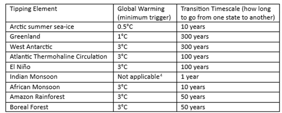
Tipping points—elements of the Earth’s climatic system that can be flipped from one state to another with a relatively minor change in temperature, and which could then cause major and abrupt changes in the climatic system itself—are a key concern for climate scientists (Lenton et al. 2023, p. 36). One of leading scientists in this field is Tim Lenton from Exeter University in the UK, and in 2008 he conducted a survey of experts on what were then regarded as the nine major and most vulnerable such tipping points—see Table 15.105F

The paper “Tipping elements in the Earth’s climate system” concluded that:

Society may be lulled into a false sense of security by smooth projections of global change. Our synthesis of present knowledge suggests that a variety of tipping elements could reach their critical point within this century under anthropogenic climate change. The greatest threats are tipping the Arctic sea-ice and the Greenland ice sheet, and at least five other elements could surprise us by exhibiting a nearby tipping point. (Lenton et al. 2008b, p. 1792. Emphasis added)

I was first alerted to the existence of this paper by a comment in Nordhaus’s manual for DICE—”Dynamic Integrated Climate and Economy”, the mathematical model he constructed by which he converts expected temperature increases into expected economic damages—in which he stated that:

The current version assumes that damages are a quadratic function of temperature change and does not include sharp thresholds or tipping points, but this is consistent with the survey by Lenton et al. (2008) (Nordhaus and Sztorc 2013, p. 11. Emphasis added)

He then elaborated in his book The Climate Casino (Nordhaus 2013) that:

There have been a few systematic surveys of tipping points in earth systems. A particularly interesting one by Lenton and colleagues examined the important tipping elements and assessed their timing… The most important tipping points, in their view, have a threshold temperature tipping value of 3°C or higher … or have a time scale of at least 300 years … Their review finds no critical tipping elements with a time horizon less than 300 years until global temperatures have increased by at least 3°C. (Nordhaus 2013, p. 60. Emphasis added)

Pardon me for stating the obvious, but Nordhaus’s reading of this paper is almost the exact opposite of what the paper actually said.

Far from the triggering of tipping points lying 300 years in the future, Lenton et al. warned that they were likely this century;106F far from a function like a quadratic, with its gradual increase in steepness as temperatures rise, being appropriate for estimating damages, they warned that such a function could lull us into “a false sense of security”; and far from 3°C of warming being required to flip tipping elements from one state to another, they asserted that much lower levels of warming would be sufficient to tip what were then seen as the two most vulnerable, Arctic summer sea-ice107F and Greenland—see Table 15—while five of the remaining seven could “surprise us by exhibiting a nearby tipping point”.

Table 15: Key Features of Tipping elements in Table 1 of (Lenton et al. 2008b, p. 1788)

I would fail any student who submitted what Nordhaus wrote as a summary of Lenton’s paper. But instead, Nordhaus was awarded the “Nobel” Prize in Economics in 2018 for his work on climate change.

If any recipient exposed the real role of this Prize, it is Nordhaus. The Economics “Nobel” Prize was not established by Alfred Nobel, and nor is it funded by the Nobel Foundation.109F It was established by the Swedish Central Bank in 1968, as a means to counter the social-democratic approach to economic policy that was popular in Sweden at the time (Offer and Söderberg 2016). Its formal name is “The Sveriges Riksbank Prize in Economic Sciences in Memory of Alfred Nobel”, and the Nobel family has been campaigning for decades, unsuccessfully, to terminate the Economics award—or to have its name trimmed to “The Sveriges Riksbank Prize”, which doesn’t implicate or piggyback on the Nobel name.110F

Given the fact that the economics departments at top-ranked Universities are dominated by Neoclassical economists, the selection process for this Prize111F means that it is awarded, not for advancing human knowledge as is the case with the real Nobels, but for defending the Neoclassical paradigm from criticism.

Here, Nordhaus did both very well, and very badly.

He did very well, because a core belief of Neoclassical economics is that market solutions are best, except where there is an “externality” in which either the costs or benefits of something are not fully captured in the market price.

Nordhaus treated climate change as an externality, and devised a market-based solution by involving a carbon price derived from what he called the “Social Cost of Carbon” (Nordhaus and Barrage 2023, p. 25). The empirical estimates he and other Neoclassical economists have made of the economic damages from global warming, versus the costs of attenuating those damages, implied that a price of $6 per ton of CO2 in 2022, rising to $90 per ton by 2040,112F would be enough to bring about the optimum balance between damages and the costs of reducing those damages. This, he asserts, would result in a temperature increase by 2100 of 2.7°C above pre-industrial temperatures, with damages to GDP in 2100 of 2.6%, compared to what GDP in 2100 would have been in the absence of global warming (Nordhaus and Barrage 2023, pp. 22-24).

He also defended Neoclassical methodology against the challenge posed by the system dynamics approach developed by Jay Forrester, and embodied both in The Limits to Growth (Meadows, Randers, and Meadows 1972) and its predecessor World Dynamics (Forrester 1971, 1973). Nordhaus not only denigrated the system dynamics approach (Nordhaus 1973, 1992a), but also developed an alternative based on the Neoclassical Ramsey Growth model (Ramsey 1928), DICE (Nordhaus 1993b). This was the world’s first “Integrated Assessment Model” (IAM), and since then, the economic analysis of climate change has been dominated by Neoclassical models—including Richard Tol’s FUND (Tol 1995) and Chris Hope’s PAGE (Hope, Anderson, and Wenman 1993)—rather than descendants of WORLD3, the system dynamics model behind the Limits to Growth.

However, Nordhaus also did very badly, because methods by which he derived empirical estimates of the economic damages from climate change were so transparently wrong that—despite my low opinion of Neoclassical economics in general—even I was shocked that these methods were accepted by referees. The referees of the “top” economics journals are exclusively Neoclassical economists, who have a similar devotion to the Neoclassical paradigm as Nordhaus, and comparable ignorance about the real world. But I was still stunned that they did not object to the bizarre empirical assumptions that Nordhaus made.

Other disciplines would not have been so forgiving. Any climate scientist would have rejected his first technique—later dubbed the “Enumerative Method” (Tol 2009, pp. 31-32)—when Nordhaus proposed it back in 1991 in “To Slow or Not to Slow: The Economics of The Greenhouse Effect” (Nordhaus 1991, pp. 930-931). Any self-respecting statistician would have rejected the second “Statistical” or “Cross-Sectional” method, which was developed by Nordhaus’s colleague Robert Mendelsohn (Mendelsohn et al. 2000).113F The “expert surveys” Nordhaus conducted (Nordhaus 1994a; Nordhaus and Moffat 2017) would likewise have been torn apart by any experienced market researcher. Subsequent variations on these themes (Burke, Hsiang, and Miguel 2015; Kahn et al. 2021; Dietz et al. 2021a) would have been rejected by any scientist with an understanding of tipping points.

These methods do not, in Solow’s colourful phrase, “pass the smell test: does this really make sense?”. But they survived refereeing because they were evaluated by advocates of Neoclassical economics who “no doubt believe what they say, but they seem to have stopped sniffing or to have lost their sense of smell altogether” (Solow 2010).

Policymakers, media, the finance sector, and much of the general public, who are unaware of what Lenton later described as the “huge gulf” (Lenton and Ciscar 2013, p. 585) between economists and climate scientists, have acted as if the economists’ estimates of damages are based on the work of scientists, and are therefore valid. As a consequence, humanity has taken trivial actions to combat climate change to date. Fossil fuel companies may have waged the war against action on climate change, but economists have been the arms dealers who have made the weapons of mass deception with which they have waged that war.

The great irony of the success of the fossil fuel disinformation campaign against action on global warming is that the weapons crafted for them by economists are so pathetically bad. I remember, before I started reading this literature, expecting to face the difficult task of explaining to a non-mathematical audience why the Ramsey growth model was the wrong foundation for modelling climate change, or why discount rates for damages should be low rather than high, and so on.114F But in fact, there was no need.

The fatal flaws in their analysis are fundamentally due to the ridiculously low estimates they have made, using ridiculously bad methods, of the damages that global warming will do to the economy. Even if the Ramsey growth models at the core of DICE, FUND, PAGE and other IAMs were perfect descriptions of reality—and they are far from that—then feeding in the numbers that economists have made up about global warming into those models would still vastly underestimate the damages that it will do to the economy. It’s all in the numbers, and the methods they’ve used to make up those numbers are statistical nonsense.

  1. Confusing the Weather with the Climate

My first exposure to the “enumerative method” was via the bland statement made about it by Tol in “The Economic Effects of Climate Change”:

Fankhauser (1994, 1995), Nordhaus (1994a), and me [sic.] (Tol, 1995, 2002a, b) use the enumerative method. In this approach, estimates of the “physical effects” of climate change are obtained one by one from natural science papers, which in turn may be based on some combination of climate models, and laboratory experiments. The physical impacts must then each be given a price and added up. For agricultural products, an example of a traded good or service, agronomy papers are used to predict the effect of climate on crop yield, and then market prices or economic models are used to value the change in output. (Tol 2009, pp. 31-32)

Superficially, this sounds like an unobjectionable method. But, as I put it in my first paper on this topic, “it’s what you don’t count that counts” (Keen 2020, p. 3). Only when I read Nordhaus’s 1991 paper “To Slow or Not to Slow: The Economics of The Greenhouse Effect” (Nordhaus 1991)—which, for no good reason, Tol did not include in his list of relevant papers115F—did I realise that the foundation of this method is assuming that climate is equivalent to the weather.

Nordhaus assumed that sectors that were “affected by climate change” would be those whose “output depends in a significant way upon climatic variables“. He then, on that assumption, assumed that fully 87% of America’s GDP would be “negligibly affected by climate change“:

Table 5 shows a sectoral breakdown of United States national income, where the economy is subdivided by the sectoral sensitivity to greenhouse warming. The most sensitive sectors are likely to be those, such as agriculture and forestry, in which output depends in a significant way upon climatic variables. At the other extreme are activities, such as cardiovascular surgery or microprocessor fabrication in ‘clean rooms’, which are undertaken in carefully controlled environments that will not be directly affected by climate change. Our estimate is that approximately 3% of United States national output is produced in highly sensitive sectors, another 10% in moderately sensitive sectors, and about 87% in sectors that are negligibly affected by climate change. (Nordhaus 1991, p. 930. Emphasis added)

The only thing that most of the industries in Nordhaus’s list of those that are “negligibly affected by climate change” have in common is that they are not directly exposed to the weather—see Table 16.

Table 16: Summary of Table 5 in (Nordhaus 1991, p. 931)

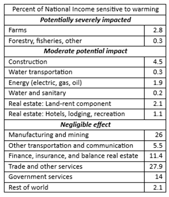
I emphasise “most”, because amongst the industries he claims will be negligibly affected is mining—some of which is open-cut, and therefore exposed to the weather.116F He reiterated this in the text of this paper:

for the bulk of the economy—manufacturing, mining, utilities, finance, trade, and most service industries—it is difficult to find major direct impacts of the projected climate changes over the next 50 to 75 years. (Nordhaus 1991, p. 932. Emphasis added)

In a sign that he really was confusing climate with weather, he amended this to underground mining in a subsequent paper—while still making the same claim that “most of the U.S. economy has little direct interaction with climate” and is therefore “unlikely to be directly affected by climate change”:

most of the U.S. economy has little direct interaction with climate… underground mining, most services, communications, and manufacturing are sectors likely to be largely unaffected by climate change—sectors that comprise around 85 percent of GDP. (Nordhaus 1993a, p. 15)

More significant though is his admission that for “the bulk of the economy” he found it “difficult to find major direct impacts of the projected climate changes over the next 50 to 75 years”.

Nordhaus found this difficult only because he is a Neoclassical economist. The obvious direct impact is humanity’s use of fossil fuels as energy sources for all the industries he thought would be “negligibly affected by climate change”. If the impacts of climate change become catastrophic for humanity as global temperatures increase, then it is feasible that energy for these industries will be curtailed, and their output will plummet. The only reason this was not obvious to him is that the Neoclassical model of production omits any role for energy, as I explained in Chapter 13.

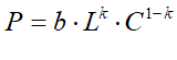
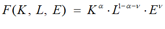
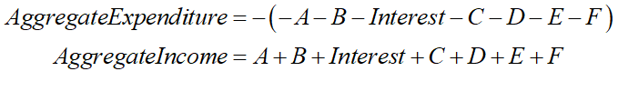
The mistake of believing that manufacturing occurs in “carefully controlled environments” is a classic example of confusing the map (the aggregate production function) with the territory (the real world). The use of an aggregate production function , in which output Y is a function F() of inputs of Labour L and Capital K, has led him to ignore, not only that energy and raw material inputs from the natural world are needed to enable factories (and offices) to function, but also that manufacturing doesn’t occur inside the brackets of a production function, but inside millions of factories, connected by the web of fossil-fuel-driven transportation systems that we have weaved across the surface of the planet. If storms destroy roads—as they did in 2022 in Canada, cutting Vancouver off from the rest of the country117F—then that web of output breaks down. All manufacturing does not occur exclusively in “carefully controlled environments”, and the millions of essential connections between the natural world and factories, and between factories themselves, have very large and direct interactions with climate.

Ignorant of all the above issues, this first use of the “enumerative method” led Nordhaus to conclude that 3°C of global warming would decrease future GDP by a mere one quarter of one percent:

We estimate that the net economic damage from a 3°C warming is likely to be around ¼% of national income for the United States in terms of those variables we have been able to quantify. This figure is clearly incomplete, for it neglects a number of areas that are either inadequately studied or inherently unquantifiable. We might raise the number to around 1% of total global income to allow for these unmeasured and unquantifiable factors, although such an adjustment is purely ad hoc. It is not possible to give precise error bounds around this figure, but my hunch is that the overall impact upon human activity is unlikely to be larger than 2% of total output. (Nordhaus 1991, pp. 932-933. Emphasis added)

Hunch“? What on earth is the word “hunch” doing in an allegedly scientific paper? And yet, in a sign of the cavalier way in which Neoclassical economists in general treat the topic of global warming, the Editor of the journal which published Nordhaus’s paper—the prestigious Economic Journal—glossed over this and many other flaws in Nordhaus’s paper, to observe that:

On the basis of the standard scientific benchmark, namely a doubling of carbon dioxide equivalent in the atmosphere, Nordhaus reaches the conclusion that climate change is likely to produce a combination of gains and losses. Moreover, he argues that there is no strong presumption of substantial net economic damages. As he points out, this does not necessarily mean that there is a strong case for inaction but rather that the arguments for intervention need to be thought through carefully. The assessment is certainly a sobering antidote to some of the more extravagant claims for the effects of global warming. (Greenaway 1991, p. 902. Boldface emphasis added)

This epitomises the attitude of Neoclassical economists in general. Lacking any understanding of the role of energy in production, mistaking the map (their model of production) for the territory (the actual system of production), and having no formal training in the physical sciences, the majority of Neoclassical economists simply don’t believe that climate change can be a significant problem. Nordhaus supplied the answer that they expected and wanted, and little critical attention was paid as to how he produced that answer.

  1. Confusing Space with Time

While it took some detective work to realise that “the enumerative method” was absurd, as I note in the previous chapter, the ludicrous nature of “the statistical approach” (also called “cross-sectional”) was obvious as soon as I saw it:

An alternative approach, exemplified in Mendelsohn’s work, can be called the statistical approach. It is based on direct estimates of the welfare impacts, using observed variations (across space within a single country) in prices and expenditures to discern the effect of climate. Mendelsohn assumes that the observed variation of economic activity with climate over space holds over time as well; and uses climate models to estimate the future effect of climate change. (Tol 2009, p. 32. Emphasis added)

The misconception that global warming over time from rising CO2 levels will have a trivial impact upon the economy, because human societies function across a wide range of climates today, is a common refrain by climate change deniers. But I was stunned to see it repeated by an academic—even if he was a Neoclassical economist. However, not only did Tol report on this approach in his paper, he defended it in numerous tweets in response to criticism by me, and by climate scientists—see Figure 61 and Figure 62.

Figure 61 : Twitter exchanges over “the statistical approach” on June 17-18 2019

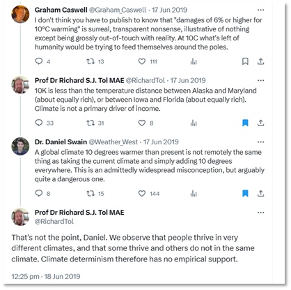
Figure 62: Twitter exchanges over “the statistical approach” on June 18 2019

There are so many ways in which this assumption—that today’s data on temperature and GDP can be used to predict the impact of global warming on the economy—that it’s hard to know where to start.

The most obvious fallacy is that space is not interchangeable with time! Despite Tol’s blasé statement that “if a relationship does not hold for climate variations over space, you cannot confidently assert that it holds over time”,118F the former cannot be used as a proxy for the latter.

If that isn’t immediately obvious to you, there are two more technical points that show this method is absurd.

The first is that the incomes of hot, temperate, and cold regions today are not independent. Hot locations, such as Florida, gain part of their income today by selling across space today to temperate places like Maryland and cold places like Alaska, and vice versa. But a future hotter Earth can’t trade across time with the colder Earth today.

To use comparisons of income variations today due to temperature differences today as a proxy for the effect of rising global temperatures on future Gross World Product, then at the very least you would need to correct for this income dependence across space, by excluding income that a hot region gains from trading with a cold region, and vice versa. Only products that are produced and consumed in cold, temperate and hot regions respectively should be used in the comparison. This would result in a much steeper relationship between temperature and income, but this was not even contemplated by the economists who used this method, let alone done.

Secondly, the mathematical term for a system which obeys Tol’s assumption—that a relationship that holds over space also holds over time—is that it is “ergodic” (Peters 2019; Drótos, Bódai, and Tél 2016). If this assumption holds, then, as the mathematician Ole Peters put it:

dynamical descriptions can often be replaced with much simpler probabilistic ones — time is essentially eliminated from the models. (Peters 2019, p. 1216)

However, ergodicity is a valid assumption only under a very restrictive set of conditions, and economists in general are unaware of this:

The conditions for validity are restrictive, even more so for non-equilibrium systems. Economics typically deals with systems far from equilibrium — specifically with models of growth… the prevailing formulations of economic theory … make an indiscriminate assumption of ergodicity. (Peters 2019, p. 1216. Emphasis added)

Using necessarily technical language, the physicists Drótos and Tél and the meteorologist Bódai are emphatic that “ergodicity does not hold” for the climate:

In nonautonomous dynamical systems, like in climate dynamics, an ensemble of trajectories initiated in the remote past defines a unique probability distribution, the natural measure of a snapshot attractor, for any instant of time, but this distribution typically changes in time. In cases with an aperiodic driving, temporal averages taken along a single trajectory would differ from the corresponding ensemble averages even in the infinite-time limit: ergodicity does not hold. (Drótos, Bódai, and Tél 2016, p. 022214-1. Emphasis added)

Therefore, you cannot, in principle, use climate across space as a proxy for climate across time. But this is what these economists did.

They also assumed, like Nordhaus before them (Nordhaus 1991), that only industries exposed to the weather would be affected by climate change: to quote Mendelsohn et al., “A separate model is designed for each sensitive market sector: agriculture, forestry, energy, water, and coastal structures” (Mendelsohn, Schlesinger, and Williams 2000, p. 39)

Finally, like Nordhaus, they simply assumed that population and economic growth in the aggregate would continue, despite a more than doubling of CO2 over pre-industrial levels (their final numerical estimates were of damages to this assumed future GDP in the absence of global warming):

We assume that humankind commits itself to a maximum equivalent CO2 concentration of 750 ppmv, which implies a carbon dioxide concentration of 612 ppmv in 2100. We assume that global population has doubled to 10 billion and that the global gross domestic product (GDP) is 217 trillion, a ten-fold increase. (Mendelsohn, Schlesinger, and Williams 2000, p. 38. Emphasis added)

With methods like these, it’s little wonder that Mendelsohn et at. predicted an even lower level of economic damages from global warming than Nordhaus generated from his “enumerative” method. They claimed that the relationship between global warming and GDP was parabolic (which Nordhaus also assumed), they described a 2.5C increase in global temperatures by 2100 as “modest”, and they predicted effectively no impact of that warming on GDP:

The climate-response functions in these studies were quadratic in temperature… Countries that are currently cooler than optimal are predicted to benefit from warming. Countries that happen to be warmer than optimal are predicted to be harmed by warming … the modest climate-change scenarios expected by 2100 are likely to have only a small effect on the world economy. The market impacts predicted in this analysis do not exceed 0.1% of global GDP and are likely to be smaller.(Mendelsohn, Schlesinger, and Williams 2000, pp. 41, 46. Emphasis added)

  1. Surveying mainly economists about Global Warming

As I noted earlier, I was alerted to existence of an expert survey of climate scientists about global warming and tipping points (Lenton et al. 2008b) by Nordhaus’s utterly false interpretations of its results (Nordhaus and Sztorc 2013, p. 11.; Nordhaus 2013, p. 60 ). This study is an exemplar of how expert surveys should be conducted.

The survey was preceded by a workshop at which the survey was trialled, after which 193 experts were identified from the literature, 52 of whom responded. Each respondent had expertise on a specific tipping point, and they were “encouraged to remain in their area of expertise” (Lenton et al. 2008a, p. 10). The key concept of “tipping elements” was carefully defined as “large elements of the planet’s climatic system (>1,000km in extent) which could be triggered into a qualitative change of state by increases in global temperature that could occur this century” (Lenton et al. 2008b, p. 1788).

Nordhaus’s paper “Expert Opinion on Climatic Change” (Nordhaus 1994b) was a caricature of this careful process. It began with a letter to three people “two experts in climatic change and one economist who had extensive experience in surveys)” (Nordhaus 1994b, p. 45), but from that point on it was biased to select economists rather than a broad range of disciplines. It ended with 19 respondents—”10 economists, four other social scientists and five natural scientists and engineers” (Nordhaus 1994b, p. 46)—but only 3 of the scientists had expertise in climate, while Nordhaus described 8 of the 10 economists as people “whose principal concerns lie outside environmental economics” (Nordhaus 1994b, p. 48)—meaning, of course, that they were not experts.119F

Furthermore, one of the scientists refused to answer Nordhaus’s key questions about the economic impact of global warming, stating that:

I must tell you that I marvel that economists are willing to make quantitative estimates of economic consequences of climate change where the only measures available are estimates of global surface average increases in temperature. As [one] who has spent his career worrying about the vagaries of the dynamics of the atmosphere, I marvel that they can translate a single global number, an extremely poor surrogate for a description of the climatic conditions, into quantitative estimates of impacts of global economic conditions. (Nordhaus 1994b, p. 51)

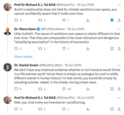
The most notable aspect of the survey was the huge gulf between the 8 non-expert economists and the two climate scientists who answered Nordhaus’s key questions. This asked for a prediction of damage to GDP in 2090 from 3°C (scenario A) and 6°C of warming (scenario C) respectively. Nordhaus noted that “Natural scientists’ estimates were 20 to 30 times higher than mainstream economists”—see Figure 63—and commented that “This difference of opinion is on the list of interesting research topics” (Nordhaus 1994b, pp. 49- 50), but this research was never done.

Figure 63: (Nordhaus 1994b, p. 49) noting the difference of opinion between climate scientists and economists

Nordhaus then used the average of the predictions from his 18 respondents as the damage prediction from this paper, thus diluting the extreme concern of 2 climate scientists in the blasé confidence of 8 non-expert economists, who were generally of the mind, as one of them put it, that:

the degree of adaptability of human economies is so high that for most of the scenarios the impact of global wanning would be “essentially zero.” (Nordhaus 1994b, p. 49)

  1. A Summing Up in 2009

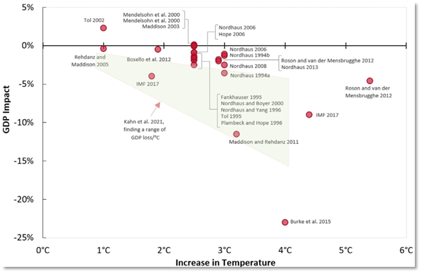
Tol summarised these results in his Table 1 (see Figure 64), and commented that “Given that the studies in Table 1 use different methods, it is striking that the estimates are in broad agreement on a number of points” (Tol 2009, p. 33). But this is spurious: the methods were all worse that suspect, all dramatically minimised the dangers, and the economists involved all shared the assumption that “exposed to climate change” meant “exposed to the weather”.

Figure 64: Table 1 from(Tol 2009, p. 31)

The real conclusion, which Tol also noted, is that these comparable predictions are a product of groupthink:

it is quite possible that the estimates are not independent, as there are only a relatively small number of studies, based on similar data, by authors who know each other well… although the number of researchers who published marginal damage cost estimates is larger than the number of researchers who published total impact estimates, it is still a reasonably small and close-knit community who may be subject to group-think, peer pressure, and self-censoring. (Tol 2009, pp. 37, 43. Emphasis added)

The groupthink continued with new methods developed by the small but growing army of economists making an academic career out of publishing estimates of economic damages from global warming. Though some of these subsequent estimates are much larger than the norm reported by Tol for studies between 1994 and 2006—of damages to future GDP of about 1-2% from 2.5°C of warming—they are still based on spurious assumptions, and estimate damages that far lower than we are likely to experience.

  1. Assuming No Change to the Climate from Global Warming

The economic study that predicts the highest damages from global warming is Burke, Hsiang, and Miguel’s 2015 paper “Global non-linear effect of temperature on economic production”: it predicts a 23% fall in global income in 2100 from a 4°C increase in global average temperature over pre-industrial levels:

If future adaptation mimics past adaptation, unmitigated warming is expected to reshape the global economy by reducing average global incomes roughly 23% by 2100. (Burke, Hsiang, and Miguel 2015. Emphasis added)

But what do they mean by the text I’ve highlighted—”If future adaptation mimics past adaptation?

They mean, in effect, that they are assuming no change to the climate from global warming. That might sound bizarre—it is bizarre—but it is a product of their method, which was to use a database of temperatures and GDP over the period from 1960-2010, and then to derive a quadratic relationship between change in temperature and GDP for the period 1960-2010. They then extrapolated this relationship forward to 2100—implicitly assuming that the increase in global temperatures from 2015 till 2100 would not make the relationship they derived from 1960-2010 data invalid.

This method was subsequently mimicked by (Kahn et al. 2021), using a later version of this database with data to 2014, to assert that “if temperature rises (falls) above (below) its historical norm by 0.01°C annually for a long period of time, income growth will be lower by 0.0543 percentage points per year” (Kahn et al. 2021). Using this relationship for data from 1960 till 2014, then then predicted that:

an increase in average global temperature of 0.04°C per year [from 2020] … reduces world’s real GDP per capita by 7.22 percent by 2100. (Kahn et al. 2021, p. 3)

The fact that this prediction was based on a linear extrapolation of the result they derived for 1960-2014 is obvious in their Figure 2—reproduced here as Figure 65.

Figure 65: Figure 2 from (Kahn et al. 2021, p. 4) showing point estimates by other economists and their range estimate

This approach, of course, ignores the impact of tipping points, which could change the structure of the planet’s atmospheric and water circulation systems completely, and make any knowledge garnered from the pre-tipping points climate irrelevant.

Fortunately for these economists, if not for human civilisation, another group of economists predicted that tipping 8 major components of the Earth’s climate—Arctic summer sea-ice, the Greenland and West Antarctic ice sheets, the Amazon rainforest, the Atlantic Meridional Overturning Circulation, permafrost, ocean methane hydrates, and the Indian monsoon—would reduce global income by a mere 1% at 3°C of warming, and 1.4% at 6°C.

  1. Reducing Tipping Points to Degrees

The paper that made this claim reached the apogee of economic delusion over climate change—though there may yet be even more absurd extensions to this literature.

The first four tipping points they consider would make Earth visibly different from space: the Arctic would be deep blue, and Greenland and the West Antarctic would be brown, rather than white; the Amazon would be brown rather than green. If the AMOC stops, the distribution of heat around the planet would be drastically altered: Western Europe and Scandinavia would be 2-5°C colder (Vellinga and Wood 2008, p. 59), while other regions would be commensurately warmer, with temperatures in South Asia rising by 2-3°C (Vellinga and Wood 2008, Figure 2, p. 50). The Permafrost and Ocean Methane Hydrates contain several times as much carbon as is currently in the atmosphere. And the lives of well over a billion people are structured around the current behaviour of the Indian monsoon.

The claim that these drastic changes to the Earth’s climatic system would cause a mere 1.4% fall in future GDP is absurd, and I and several colleagues, including the climate scientist Tim Lenton, said so in a letter to Proceedings of the National Academy of Sciences, the journal that published this paper (Keen et al. 2022). In a sign of just how disconnected from reality climate economists are, the authors of this study were surprised that we thought that impacts would be larger:

Keen et al. argue the conclusions and procedures in ref. 2 do not make sense, seemingly taking it as given that the economic impacts of climate tipping points will be larger than our estimates. (Dietz et al. 2022. Emphasis added)

They also defended themselves with the claim that “Dietz et al. modeling of climate tipping points is informative even if estimates are a probable lower bound” (Dietz et al. 2022).

These comments show how apt Robert Solow’s comment was, after the “Global Financial Crisis”, that many economists seem have lost their sense of smell (Solow 2010), and can make statements that are obviously nonsense, but not see that themselves.

A 1.4% fall of future GDP is only marginally greater than no fall at all. Normal people—that is, anyone who is neither a Neoclassical economist nor a climate change denier—would guess that climatic effects as severe as this paper contemplated would mean 100% destruction of the economy, not zero. It is in no way useful today to say that the fall in GDP will be 1.4%, rather than zero—there’s virtually no difference between them. Instead, this feeds into the delusions already built into this literature, that climate change is a minor issue, by portraying the most dangerous aspect of climate change—tipping points—as an equally trivial problem.

Dietz et al. also asserted that the impact of tipping points can be modelled using a “second-order polynomial”:

Tipping points increase the temperature response to GHG emissions over most of the range of temperatures attained … Using a second-order polynomial to fit the data, 2 warming in the absence of tipping points corresponds to 2.3 warming in the presence of tipping points, for instance. … Tipping points reduce global consumption per capita by around 1% upon 3 warming and by around 1.4% upon 6 warming, based on a second-order polynomial fit of the data. (Dietz et al. 2021a, p. 5. Emphasis added)

For non-mathematical readers, a second order polynomial (AKA a “quadratic”) asserts that the value of one variable is equal to a constant, multiplied by the value of another variable squared. In this case, economic damages are alleged to be equal to a constant multiplied by the increase in global average temperature squared.

As I discuss in the next section, this is an inappropriate function to use for modelling global warming in general. But it is particularly inappropriate here, since it contradicts the formal definition of a tipping point given by scientists in “Tipping elements in the Earth’s climate system” (Lenton et al. 2008b):

a system is a tipping element if the following condition is met: 1. The parameters controlling the system can be transparently combined into a single control … , and there exists a critical control value … from which any significant variation … leads to a qualitative change … in a crucial system feature … (Lenton et al. 2008b, p. 1786)120F

In the case of tipping points triggered by global warming, the control is the global average temperature, and the critical control value is the temperature at which the state of the tipping point, say the Arctic Ocean,121F is altered from one state to another—in this example, from ice-covered during summer to ice-free. The qualitative change is that a surface which used to reflect 90% of sunlight now absorbs 90%, and hence changes from cooling the planet to warming it.

To emulate this with a smooth mathematical function, at the very least you need a function whose rate of acceleration increases as global temperatures increase past the critical level. A quadratic cannot do this, since the rate of acceleration of a quadratic never changes.

Regardless, using this paper, Nordhaus is now claiming that he has incorporated the impact of tipping points in DICE:

Second, we have added the results of a comprehensive study of tipping points (Dietz et al. 2021), which estimates an additional 1% loss of global output due to 3 °C warming. (Nordhaus and Barrage 2023, pp. 8-9).

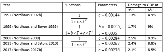
He has done this mainly by increasing the single parameter in his quadratic damage function from 0.00227 to 0.003467, thus resulting in a small increase in expected damages—rather than the catastrophic impacts rightly anticipated by climate scientists. This is the first time since 1992 that he has increased the value of his damage parameter—see Table 17—but this in no way accounts for tipping points.

  1. Assuming Constant Acceleration in Economic Damages

Nordhaus’s damage function has taken different forms over the life of DICE from 1992 till 2023—see Table 17 for its various incarnations—but the fundamental assumption has remained that economic damages from global warming will be proportional to the temperature change squared. Table 17 shows the form this function has taken, the parameters, and the predicted damages these functions return at 3°C and 6°C increases over pre-industrial levels.

Table 17: The damage function in Nordhaus’s DICE over time

This practice is rife amongst Neoclassical climate change economists, and it has absolutely no empirical or theoretical justification. In fact, this is one aspect of their modelling which has been consistently criticized by other economists—and in language similar to mine, rather than the anodyne norms of academic discourse:

Numerous subjective judgements, based on fragmentary evidence at best, are incorporated in the point estimate of 1.8% damages at 2.5°C … The assumption of a quadratic dependence of damage on temperature rise is even less grounded in any empirical evidence. Our review of the literature uncovered no rationale, whether empirical or theoretical, for adopting a quadratic form for the damage function—although the practice is endemic in IAMs. (Stanton, Ackerman, and Kartha 2009, p.172. Emphasis added)

Modelling climate economics requires forecasts of damages at temperatures outside historical experience; there is no reason to assume a simple quadratic (or other low-order polynomial) damage function. (Stanton, Ackerman, and Kartha 2009, p.179. Emphasis added)

this damage function is made up out of thin air. It isn’t based on any economic (or other) theory or any data. Furthermore, even if this inverse quadratic function were somehow the true damage function, there is no theory or data that can tell us the values for the parameters. (Pindyck 2017, p. 104. Emphasis added)

This paper asks how much we might be misled by our economic assessment of climate change when we employ a conventional quadratic damages function and/or a thin-tailed probability distribution for extreme temperatures… These numerical exercises suggest that |we might be underestimating considerably the welfare losses from uncertainty by using a quadratic damages function. (Weitzman 2012, p. 221)

Despite this criticism, Neoclassical climate change economists persist in using such a simple and misleading function: they acknowledge, and then ignore, their critics. In manual for the latest version of DICE, Nordhaus blandly states that:

Based on recent reviews, we further assume that a quadratic damage function best captures the impact of climate change on output (Nordhaus and Moffat, 2017; Hsiang et al., 2017). (Nordhaus and Barrage 2023, p. 8. Emphasis added)

But these “reviews” were by other economists who are just as deluded as Nordhaus, and considered statistical regressions of change in temperature data today against GDP today—in other words, they were based on the fallacy that today’s variations in climate and income across space can be used to predict the consequences climate change over time on the global economy.

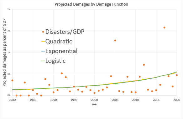
To illustrate just how misleading this assumption is, Brian Hanley and I decided to compare a quadratic damage function to an exponential and a logistic function in (Keen and Hanley 2023).123F The data to which we fitted these functions was the USA’s National Oceanic and Atmospheric Administration (NOAA) Billion Dollar Damages Database.124F Across the actual range of recorded data, the functions are indistinguishable: despite appearances, there are 3 lines in Figure 66, not just one.

Figure 66: The fit of quadratic, exponential and logistic functions to the NOAA Billion Dollar Damages database

However, when you extrapolate those functions forward, the outcome is dramatically different. The quadratic extrapolation predicts damages within the ballpark set by Nordhaus and his acolytes, of a roughly 10% fall in future GDP by 2100. But the logistic suggests complete destruction of GDP in 2100, while the exponential implies that human civilisation will end by 2080—see Figure 67.

Figure 67: The extrapolation of quadratic, exponential and logistic functions from the NOAA Billion Dollar Damages database

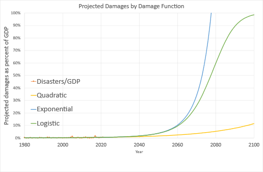
Neither of our “predictions” are meant as such: we dispute the very concept of finding the fingerprint of global warming in current data. But if you are going to undertake that experiment, then at least do it with reliable 3rd party data like NOAA’s database, rather than numbers you’ve made up yourselves—as economists have done. And don’t only fit functions to your “data” which by assumption assert that global warming can’t be a problem—as economists have done by persisting with quadratic damage functions.

Of course, the longer you wait, the more likely you are to find evidence of global warming in current economic damages. The whole point of climate change research—before it was hijacked by economists—was to avoid this experience in the first place, by giving humanity sufficient warning to change its ways and avoid catastrophe. Now, thanks to the appallingly bad work by economists, and its success in persuading politicians that global warming is a problem of the 22nd century rather than the 21st, we are highly likely to experience that catastrophe—and in the immediate rather than the far distant future.

  1. Modelling Weather without Precipitation

Another sign of the cavalier way economists have treated climate change is that their “Integrated Assessment Models” (IAMs) include the impact of temperature on the economy, but not precipitation. Dietz et al. note, when explaining the results of the study they used to assess the impact of losing the AMOC on the economy, that:

AMOC slowdown is expected to have physical effects other than temperature change, for instance effects on precipitation and regional sea levels, but these have yet to be incorporated in economic studies. (Dietz et al. 2021b, p. 25. Emphasis added)

This is an outrageous failing: it has been more than 30 years since the first IAM, Nordhaus’s DICE, was published in 1992 (Nordhaus 1992b). And yet no economist has yet tried to include rainfall in addition to temperature in his—they are exclusively men—model of global warming!125F

This failing lies behind possibly the most ridiculous claim in this literature, that losing the Atlantic Meridional Overturning Circulation—which is part of the planet-spanning “Thermohaline Circulation” (THC)—will actually boost the economy. This came from a study using Tol’s IAM “FUND”, in which the authors claimed that:

If the THC slows down a little, the global impact is a positive 0.2-0.3 percent of income. This goes up to 1.3 percent for a more pronounced slowdown. (Anthoff, Estrada, and Tol 2016, p. 604. Emphasis added)

This is nonsense, as was pointed out when actual climate scientists tackled the same issue using their far more sophisticated GCMs. In a study for the OECD, which considered the impact of the collapse of the AMOC in conjunction with a 2.5°C rise in temperature, Lenton concluded that this would cause a 70% fall in the proportion of the planet’s land surface that is suitable for growing corn and wheat. Far from having a positive impact on income, he stated that:

an AMOC collapse would clearly pose a critical challenge to food security. Such a collapse combined with climate change would have a catastrophic impact. (OECD 2021, p. 151. Emphasis added)

Tol and his colleagues waved away their failure to include the impact of precipitation changes in their paper with the statement that “Integrated assessment models often assume that other climate variables scale with temperature” (Anthoff, Estrada, and Tol 2016, p. 605. Emphasis added). In plain English, this is the assumption that, if temperature “gets better”, then so does rainfall! Since an AMOC shutdown would counteract global warming for northern Europe and North America, and they are the biggest economies, ipso facto the global economy will improve from losing this fundamental component of the planet’s climate.

This is nonsense: changes in global and local temperatures will cause changes in global and local precipitation, but by no means will they be in the same qualitative direction: a change to a more pleasant local temperature could be accompanied by the region turning into a desert or a swamp from decreased or increased rainfall.

This dissembling language is typical of Neoclassical climate change economics, with the most egregious but effective example being how they state damages as a percentage fall in future GDP.

  1. The Shell and Pea Trick of Damages to Future GDP

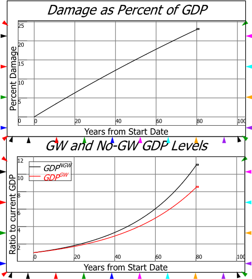
The biggest damage estimate in this literature comes from Burke et al.’s paper “Global non-linear effect of temperature on economic production”, which asserted that a 4°C increase in global temperature by 2100 would cause future GDP to fall by almost 25%:

unmitigated warming is expected to reshape the global economy by reducing average global incomes roughly 23% by 2100. (Burke, Hsiang, and Miguel 2015, p. 235)

That sounds like a big number, but it implies a trivial fall in the rate of economic growth. If the expected growth rate without global warming was 3% per annum, then this most severe damage prediction in the Neoclassical climate change literature asserts that global warming will reduce the annual rate of economic growth by 0.33% per annum, to 2.67% per year. Therefore, rather than GDP in 2100 being 11 times larger than 2020 in 2020, it will be “only” 8.5 times—see Figure 68.

Figure 68: Burke et al.’s 23% fall in GDP in 2100 graphed against time

The superficially intelligent reaction to this prediction is the one given by Stuart Kirk in his (in)famous speech at the Financial Times conference in 2022 entitled “Why investors need not worry about climate risk”
126F where, in reference to a hypothetical 5% fall in GDP by 2100, he said “who cares, you will never notice”:

Even by the UN IPCC own numbers, climate change will have a negligible effect on the world economy. A (large) temperature rise of 3.6 degrees by 2100 means a loss of 2.6 percent of global GDP. Let’s assume 5%… What they fail to tell everybody of course is between now and 2100 economies are going to grow a lot. At about 2 percent it’s [500%] and about three percent it’s [1000%] … the world is going to be between 500 or 1000 percent richer. If you knock five percent off that in 2100 who cares? You will never notice.

This is indeed how most politicians, policymakers, journalists, and much of the public, have actually reacted: Kirk is exceptional only for voicing this attitude.

However, the deeply intelligent reaction to these predictions is “why do economists expect such trivial damages from climate change?”. If, rather than predicting “a 23% fall in GDP in 2100” from 4°C of warming, economists said “a 0.33% fall in the annual rate of economic growth”, the triviality of their estimates might have alerted scientists to the fact that economists really don’t understand what climate change is.

The “x% fall in GDP by the year yyyy” predictions of climate economists can be converted into a “change in the annual growth rate of x%” prediction by the simple formula:

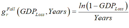
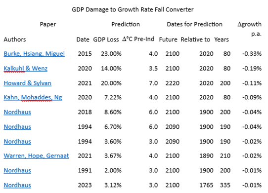
Here GDPLoss represents the fall in future GDP predicted by economists (stated as a decimal rather than a percentage), and Years is how far in the future this prediction was with respect to a reference date. Table 18 applies this formula to some of the roughly 40 papers economists have written that have generated fall in future GDP predictions, and converts them into predicted falls in the annual rate of growth. Not one of them implies a decline in GDP from climate change, and many are predictions of a decline in the rate of growth which is below the 0.1% per year accuracy with which actual GDP growth is measured today.

Table 18: Some economic damage estimates converted into predicted fall in annual growth rate

These figures explain why one of Nordhaus’ respondents to his 1994 survey of “experts” remarked that:

“I am impressed with the view that it takes a very sharp pencil to see the difference between the world with and without climate change or with and without mitigation.” (Nordhaus 1994b, p. 48)

  1. Conclusion

The only explanation for how bad this work by Neoclassical climate change economists has been is the methodological topic covered in the previous chapter: consciously or otherwise, Neoclassical economists respond to a perceived attack on their paradigm by making domain assumptions that appear reasonable to them, but are insane from any outsider’s perspective. The paradigm is preserved, at the expense, when these crazy assumptions affect government policy, of harming the economy itself.

In the past, as with the Global Financial Crisis, this has simply meant that economists have blinded policymakers to economic events like the Great Depression and the Global Financial Crisis, where a corrective action by governments could ultimately attenuate the damage. But with Global Warming, their defence of their paradigm will in all likelihood put capitalism into an existential crisis. The damages from climate change will be far, far greater than economists have told policymakers they will be, and the remedies are not relatively simple economic policies like The New Deal, but engineering feats that humanity has never managed in the past, and which may be too little, too late, against the enormous forces of a perturbed climate.

Therefore, Neoclassical economics is not merely an inappropriate paradigm for the analysis of capitalism, but a deluded manner of thinking about capitalism that may end up causing the destruction of capitalism itself.

It has to go.

  1. References

    Anthoff, David, Francisco Estrada, and Richard S. J. Tol. 2016. ‘Shutting Down the Thermohaline Circulation’, The American Economic Review, 106: 602-06.

    Burke, Marshall, Solomon M. Hsiang, and Edward Miguel. 2015. ‘Global non-linear effect of temperature on economic production’, Nature, 527: 235.

    Dietz, Simon, James Rising, Thomas Stoerk, and Gernot Wagner. 2021a. ‘Economic impacts of tipping points in the climate system’, Proceedings of the National Academy of Sciences, 118: e2103081118.

    ———. 2021b. ‘Economic impacts of tipping points in the climate system: supplementary information’, Proceedings of the National Academy of Sciences, 118: e2103081118.

    ———. 2022. ‘Reply to Keen et al.: Dietz et al. modeling of climate tipping points is informative even if estimates are a probable lower bound’, Proceedings of the National Academy of Sciences, 119: e2201191119.

    Drótos, Gábor, Tamás Bódai, and Tamás Tél. 2016. ‘Quantifying nonergodicity in nonautonomous dissipative dynamical systems: An application to climate change’, Physical review. E, 94: 022214.

    Forrester, Jay W. 1971. World Dynamics (Wright-Allen Press: Cambridge, MA).

    ———. 1973. World Dynamics (Wright-Allen Press: Cambridge, MA).

    Greenaway, D. 1991. ‘Economic Aspects Of Global Warming: Editorial Note’, The Economic journal (London), 101: 902-03.

    Hanley, Brian P., and Stephen Keen. 2022. “The Sign of Risk for Present Value of Future Losses.” In arXiv.

    Hope, Chris, John Anderson, and Paul Wenman. 1993. ‘Policy analysis of the greenhouse effect: An application of the PAGE model’, Energy Policy, 21: 327-38.

    Kahn, Matthew E., Kamiar Mohaddes, Ryan N. C. Ng, M. Hashem Pesaran, Mehdi Raissi, and Jui-Chung Yang. 2021. ‘Long-term macroeconomic effects of climate change: A cross-country analysis’, Energy Economics: 105624.

    Keen, S., and Brian P. Hanley. 2023. “Supporting Document to the DICE against pensions: how did we get here?” In. London: Carbon Tracker.

    Keen, Steve. 2020. ‘The appallingly bad neoclassical economics of climate change’, Globalizations: 1-29.

    Keen, Steve, Timothy Lenton, T. J. Garrett, James W. B. Rae, Brian P. Hanley, and M. Grasselli. 2022. ‘Estimates of economic and environmental damages from tipping points cannot be reconciled with the scientific literature’, Proceedings of the National Academy of Sciences, 119: e2117308119.

    Lenton, Timothy, David I. Armstrong McKay, Sina Loriani, Jesse F. Abrams, Steven J. Lade, Jonathan F. Donges, Manjana Milkoreit, Tom Powell, S.R. Smith, Caroline Zimm, J.E. Buxton, Emma Bailey, L. Laybourn, A. Ghadiali, and J.G. Dyke. 2023. “The Global Tipping Points Report 2023 ” In. Exeter, UK.: University of Exeter.

    Lenton, Timothy, and Juan-Carlos Ciscar. 2013. ‘Integrating tipping points into climate impact assessments’, Climatic Change, 117: 585-97.

    Lenton, Timothy M., Hermann Held, Elmar Kriegler, Jim W. Hall, Wolfgang Lucht, Stefan Rahmstorf, and Hans Joachim Schellnhuber. 2008a. ‘Supplement to Tipping elements in the Earth’s climate system’, Proceedings of the National Academy of Sciences, 105.

    ———. 2008b. ‘Tipping elements in the Earth’s climate system’, Proceedings of the National Academy of Sciences, 105: 1786-93.

    Meadows, Donella H., Jorgen Randers, and Dennis Meadows. 1972. The limits to growth (Signet: New York).

    Mendelsohn, Robert, Wendy Morrison, Michael Schlesinger, and Natalia Andronova. 2000. ‘Country-Specific Market Impacts of Climate Change’, Climatic Change, 45: 553-69.

    Mendelsohn, Robert, Michael Schlesinger, and Larry Williams. 2000. ‘Comparing impacts across climate models’, Integrated Assessment, 1: 37-48.

    Nordhaus, William. 1994a. ‘Expert Opinion on Climate Change’, American Scientist, 82: 45–51.

    ———. 2008. ‘Results of the DICE-2007 Model Runs.’ in, A Question of Balance (Yale University Press).

    ———. 2013. The Climate Casino: Risk, Uncertainty, and Economics for a Warming World (Yale University Press: New Haven, CT).

    ———. 2018. ‘Projections and Uncertainties about Climate Change in an Era of Minimal Climate Policies’, American Economic Journal: Economic Policy, 10: 333–60.

    Nordhaus, William D. 1973. ‘World Dynamics: Measurement Without Data’, The Economic Journal, 83: 1156-83.

    ———. 1991. ‘To Slow or Not to Slow: The Economics of The Greenhouse Effect’, The Economic Journal, 101: 920-37.

    ———. 1992a. ‘Lethal Model 2: The Limits to Growth Revisited’, Brookings Papers on Economic Activity: 1-43.

    ———. 1992b. ‘An Optimal Transition Path for Controlling Greenhouse Gases’, Science, 258: 1315-19.

    ———. 1993a. ‘Reflections on the Economics of Climate Change’, The Journal of Economic Perspectives, 7: 11-25.

    ———. 1993b. ‘Rolling the ‘DICE’: an optimal transition path for controlling greenhouse gases’, Resource and Energy Economics, 15: 27-50.

    ———. 1994b. ‘Expert Opinion on Climatic Change’, American Scientist, 82: 45-51.

    ———. 2017a. ‘Revisiting the social cost of carbon’, Proceedings of the National Academy of Sciences, 114: 1518-23.

    ———. 2017b. ‘Revisiting the social cost of carbon Supporting Information’, Proceedings of the National Academy of Sciences, 114: 1-2.

    Nordhaus, William D., and Lint Barrage. 2023. “Policies, Projections, And The Social Cost Of Carbon: Results From The Dice-2023 Model.” In. Cambridge, MA: National Bureau Of Economic Research.

    Nordhaus, William D., and Joseph G. Boyer. 1999. ‘Requiem for Kyoto: An Economic Analysis of the Kyoto Protocol’, The Energy Journal, 20: 93-130.

    Nordhaus, William D., and Andrew Moffat. 2017. “A Survey Of Global Impacts Of Climate Change: Replication, Survey Methods, And A Statistical Analysis.” In. New Haven, Connecticut: Cowles Foundation.

    Nordhaus, William, and Paul Sztorc. 2013. “DICE 2013R: Introduction and User’s Manual.” In.

    OECD. 2021. Managing Climate Risks, Facing up to Losses and Damages.

    Offer, Avner, and Gabriel Söderberg. 2016. The Nobel Factor: The Prize in Economics, Social Democracy, and the Market Turn (Princeton University Press: New York).

    Peters, Ole. 2019. ‘The ergodicity problem in economics’, Nature Physics, 15: 1216-21.

    Pindyck, Robert S. 2017. ‘The Use and Misuse of Models for Climate Policy’, Review of Environmental Economics and Policy, 11: 100-14.

    Piontek, Franziska, Laurent Drouet, Johannes Emmerling, Tom Kompas, Aurélie Méjean, Christian Otto, James Rising, Bjoern Soergel, Nicolas Taconet, and Massimo Tavoni. 2021. ‘Integrated perspective on translating biophysical to economic impacts of climate change’, Nature Climate Change, 11: 563-72.

    Ramsey, F. P. 1928. ‘A Mathematical Theory of Saving’, The Economic Journal, 38: 543-59.

    Solow, R. M. 2010. “Building a Science of Economics for the Real World.” In House Committee on Science and Technology Subcommittee on Investigations and Oversight. Washington.

    Stanton, Elizabeth A., Frank Ackerman, and Sivan Kartha. 2009. ‘Inside the integrated assessment models: Four issues in climate economics’, Climate and Development, 1: 166-84.

    Tol, R. S. J. 1995. ‘The damage costs of climate change toward more comprehensive calculations’, Environmental and Resource Economics, 5: 353-74.

    Tol, Richard S. J. 2009. ‘The Economic Effects of Climate Change’, The Journal of Economic Perspectives, 23: 29–51.

    Vellinga, Michael, and Richard A. Wood. 2008. ‘Impacts of thermohaline circulation shutdown in the twenty-first century: Abrupt Climate Change Near the Poles’, Climatic Change, 91: 43-63.

    Weitzman, Martin L. 2012. ‘GHG Targets as Insurance Against Catastrophic Climate Damages’, Journal of Public Economic Theory, 14: 221-44.

Capitalism, with friends like these, you don’t need enemies

Though I have been interested in ecological economics ever since I read The Limits to Growth (Meadows, Randers, and Meadows 1972), E.F. Schumacher (Schumacher 1973, 1979) and Hermann Daly (Daly 1974) in the early 1970s, and I have been a critic of Neoclassical economics for just as long, I didn’t start critiquing the Neoclassical approach to climate change until 2019. This was because, though I expected it to be bad, I felt that I could not critique it until after I had made a positive contribution to ecological economics myself.

This is a chapter in my draft book Rebuilding Economics from the Top Down, which will be published early in 2024 by the Budapest Centre for Long-Term Sustainability

If you like my work, please consider becoming a paid subscriber from as little as $10 a year on Patreon, or $5 a month on Substack

That occurred when, while working with the brilliant pioneer of the economics of energy Bob Ayres, the aphorism “labour without energy is a corpse, while capital without energy is a sculpture” occurred to me, and enabled me to work out how to bring energy into mathematical models of production in a fundamental way, using the concepts explained in the last chapter. In June 2019, after our paper “A Note on the Role of Energy in Production” (Keen, Ayres, and Standish 2019, p. 41) had been published—and after William Nordhaus had been awarded the “Nobel” Prize in Economics in 2018 for his work on the economics of climate change—I sat down to read the Neoclassical literature, commencing with Richard Tol’s overview paper “The Economic Effects of Climate Change” (Tol 2009).

Minutes later, I read the sentences quoted below, and I was both horrified, and very regretful of my decision to delay taking this area on:

An alternative approach, exemplified in Mendelsohn’s work, can be called the statistical approach. It is based on direct estimates of the welfare impacts, using observed variations (across space within a single country) in prices and expenditures to discern the effect of climate. Mendelsohn assumes that the observed variation of economic activity with climate over space holds over time as well; and uses climate models to estimate the future effect of climate change. (Tol 2009, p. 32. Emphasis added)

This assumption was patently absurd—as I explain in the next chapter—and yet it had been published in a “top five” economics journal (Bornmann, Butz, and Wohlrabe 2018; Mixon and Upadhyaya 2022). Worse, as I read the literature in detail, I found that, though many other aspects of the Neoclassical economics of climate change had been criticized by other economists, (Kaufmann 1997, 1998; Darwin 1999; Quiggin and Horowitz 1999; DeCanio 2003; Schlenker, Hanemann, and Fisher 2005; Ackerman and Stanton 2008; Stanton, Ackerman, and Kartha 2009; Ackerman, Stanton, and Bueno 2010; Weitzman 2011b, 2011a; Ackerman and Munitz 2012; Pindyck 2013, 2017), no-one had criticised it for what I saw as its most obvious flaw: the simply ludicrous “data” to which Neoclassical models of climate change had been fitted.

The empirical assumptions that economists specialising in climate change have made are so—to be frank—stupid, that, even if their mathematical models perfectly captured the actual structure of the global economy precisely (which of course they don’t), their forecasts of economic damages from climate change would still be ludicrously low. They are also so obviously wrong that the mystery is why these assumptions were ever published. Therefore, before I discuss their work on climate change, I have to take a diversion into the topics of scientific and economic methodology.

  1. “Simplifying Assumptions”, Milton Friedman, and the “F-twist”

As I noted in Chapter 5, every survey that has ever been done of the cost structure of real-world firms has returned a result that contradicts Neoclassical economic theory. Rather than firms facing rising marginal cost because of diminishing marginal productivity, the vast majority of real-world firms operate with substantial excess capacity, and therefore experience constant or even rising marginal productivity as production increases. This means that marginal cost either remains constant or falls with output, rather than rising, as mainstream economic theory assumes.

In the 1930s, 40s and early 50s, a large number of papers were published reporting on these results in the leading journals of the discipline, such as Oxford Economic Papers (Hall and Hitch 1939; Tucker 1940; Andrews 1941, 1949, 1950; Andrews and Brunner 1950), the Quarterly Journal of Economics (Eiteman 1945), and the American Economic Review (Means 1936; Tucker 1937; Garver et al. 1938; Tucker 1938; Lester 1946; Oliver 1947; Eiteman 1947; Lester 1947; Eiteman 1948; Eiteman and Guthrie 1952; Eiteman 1953). These papers made the point that, since marginal cost is either constant or falling, the mainstream profit-maximisation rule, of equating marginal revenue to marginal cost, must be wrong.

Writing in the American Economic Review, Eiteman put it this way in 1947: an engineer designs a factory:

so as to cause the variable factor to be used most efficiently when the plant is operated close to capacity. Under such conditions an average variable cost curve declines steadily until the point of capacity output is reached. A marginal curve derived from such an average cost curve lies below the average curve at all scales of operation short of peak production, a fact that makes it physically impossible for an enterprise to determine a scale of operations by equating marginal cost and marginal revenues unless demand is extremely inelastic. (Eiteman 1947, p. 913. Emphasis added)

One might have expected that economists would have reacted to this empirical discovery by realising that economic theory had to change. But instead, in “The Methodology of Positive Economics” (Friedman 1953`), Milton Friedman argued that economists should ignore these papers, and criticism of economics for being unrealistic in general, on the basis that the more significant a theory was, the more “unrealistic” its assumptions would be—an argument that Samuelson dubbed “The F-twist” (Archibald, Simon, and Samuelson 1963; Wong 1973):

In so far as a theory can be said to have “assumptions” at all, and in so far as their “realism” can be judged independently of the validity of predictions, the relation between the significance of a theory and the “realism” of its “assumptions” is almost the opposite of that suggested by the view under criticism. Truly important and significant hypotheses will be found to have “assumptions” that are wildly inaccurate descriptive representations of reality, and, in general, the more significant the theory, the more unrealistic the assumptions (in this sense). The reason is simple. A hypothesis is important if it “explains” much by little, that is, if it abstracts the common and crucial elements from the mass of complex and detailed circumstances surrounding the phenomena to be explained and permits valid predictions on the basis of them alone. To be important, therefore, a hypothesis must be descriptively false in its assumptions… (Friedman 1953, p. 14. Emphasis added)

He followed up with an attack on the significance of the papers which pointed out that marginal cost does not rise with output (as well as an attack on the model of imperfect competition):

The theory of monopolistic and imperfect competition is one example of the neglect in economic theory of these propositions. The development of this analysis was explicitly motivated, and its wide acceptance and approval largely explained, by the belief that the assumptions of “perfect competition” or, “perfect monopoly” said to underlie neoclassical economic theory are a false image of reality. And this belief was itself based almost entirely on the directly perceived descriptive inaccuracy of the assumptions rather than on any recognized contradiction of predictions derived from neoclassical economic theory. The lengthy discussion on marginal analysis in the American Economic Review some years ago is an even clearer, though much less important, example. The articles on both sides of the controversy largely neglect what seems to me clearly the main issue—the conformity to experience of the implications of, the marginal analysis—and concentrate on the largely irrelevant question whether businessmen do or do not in fact reach their decisions by consulting schedules, or curves, or multivariable functions showing marginal cost and marginal revenue. (Friedman 1953, p. 15. Emphasis added)

Friedman ridiculed the survey methods behind this research:

The abstract methodological issues we have been discussing have a direct bearing on the perennial criticism of “orthodox” economic theory as “unrealistic”… A particularly clear example is furnished by the recent criticisms of the maximization-of-returns hypothesis on the grounds that businessmen do not and indeed cannot behave as the theory “assumes” they do. The evidence cited to support this assertion is generally taken either from the answers given by businessmen to questions about the factors affecting their decisions—a procedure for testing economic theories that is about on a par with testing theories of longevity by asking octogenarians how they account for their long life—or from descriptive studies of the decision-making activities of individual firms. Little if any evidence is ever cited on the conformity of businessmen’s actual market behaviour—what they do rather than what they say they do—with the implications of the hypothesis being criticized, on the one hand, and of an alternative hypothesis, on the other. (Friedman 1953, pp. 30-31. Emphasis added)

And he also ridiculed the search for more realism in general:

A theory or its “assumptions” cannot possibly be thoroughly “realistic” in the immediate descriptive sense so often assigned, to this term. A completely “realistic” theory of the wheat market would have to include not only the conditions directly underlying the supply and demand for wheat but also the kind of coins or credit instruments used to make exchanges; the personal characteristics of wheat-traders such as the color of each trader’s hair and eyes, his antecedents and education, the number of members of his family, their characteristics, antecedents, and education, etc.; the kind of soil on which the wheat was grown, its physical and chemical characteristics, the weather prevailing during the growing season; the personal characteristics of the farmers growing the wheat and of the consumers who will ultimately use it; and so on indefinitely. Any attempt to move very far in achieving this kind of “‘realism” is certain to render a theory utterly useless. (Friedman 1953, p. 32)

Friedman’s paper merely codified the standard retort that economists have always made when their assumptions have been challenged, but since his paper, he has been cited as the authority when needed. However, his paper had a definite if perverse effect on the development of Neoclassical theory: though he cautioned in a footnote that “The converse of the proposition does not of course hold: assumptions that are unrealistic (in this sense) do not guarantee a significant theory”, his claim almost led to an arms race amongst economists to make the most unrealistic assumptions possible.

  1. Domain Assumptions, Paradigms, and Scientific Revolutions

In the paper “‘Unreal Assumptions’ in Economic Theory: The F‐Twist Untwisted” (Musgrave 1981), the philosopher Alan Musgrave explained that Friedman’s dictum was true of “simplifying assumptions”, but utterly false when applied to what he called “domain assumptions”.

A simplifying assumption is a decision to omit some aspect of the real world which, if you included it, would make your model vastly more complicated, but only change your results very slightly. The items Friedman lists in his example of a “completely “realistic” theory of the wheat market” are unrealistic instances of this: an economic model including “the color of each trader’s hair and eyes” would be vastly more complicated, and would obviously have no effect on the model’s predictive power, but why would anyone bother creating such a model?

A more realistic example of a simplifying assumption is Galileo’s apocryphal proof that objects of different weight fall at the same speed by dropping lead balls out of the Leaning Tower of Pisa. Such an experiment “assumes” that the balls are being dropped in a vacuum. Taking air resistance into account would result in a vastly more complicated experiment, but the result would be much the same, because given the height of the Leaning Tower of Pisa, and the density and weight of lead balls, the simplifying assumption that the existence of air resistance can be ignored is reasonable.

But a domain assumption is completely different: this is an assumption which determines whether your model applies or not. If your domain assumption applies, then your theory also applies, and is valid; if it does not, then your theory does not apply and is invalid. Therefore, domain assumptions should be realistic, otherwise the resulting theory will be false. Realism in domain assumptions is essential.

This is why the target of Friedman’s ire is so important: he was defending, not a simplifying assumption, but a domain assumption which is false.

The Neoclassical theory of profit maximisation—that a firm maximizes profit by equating marginal cost and marginal revenue—applies if firms have rising marginal cost. However, the papers that Friedman advised economists not to read revealed that, for the vast majority of firms, marginal cost did not rise, and for the reasons given by Eiteman earlier: factories are designed by engineers to be most efficient at maximum output. As the mathematics in Chapter 5 showed, in this real-world situation, marginal revenue is always greater than marginal cost, and the sensible profit maximisation strategy is to sell as many units as possible. Making the domain assumption that real-world factories experience diminishing marginal productivity (and therefore rising marginal cost) is a domain assumption which leads to a false theory of profit maximisation for the real world.

This is why the results of Blinder’s survey were, as Alan Blinder put it, “overwhelmingly bad news … (for economic theory) (Blinder 1998, p. 102), because the theory of supply and demand falls apart:

  • There is no supply curve: as Blinder acknowledges, rising marginal cost is “enshrined in every textbook and employed in most economic models. It is the foundation of the upward-sloping supply curve” (Blinder 1998, p. 101).
  • Though sales necessarily equal purchases, this is not a point of equilibrium: the sellers have excess capacity and could sell more units if they could find buyers.
  • The welfare-maximising conclusions of Neoclassical economics also fall by the wayside: rather than the market equating marginal revenue and marginal cost, thus maximising consumer utility subject to the constraints of producer cost, there is a gap between the two that explains the evolutionary competitive process we actually see in the real world.
  • That competitive struggle leads to a power law distribution of firm sizes—which again, we see in the real world (Axtell 2001, 2006). Perfect competition is not a desirable state, but a myth. A very different—and much richer—theory is required to understand actual competition and actual microeconomic behaviour than the toy models of Neoclassical economics.

Acknowledging this empirical research into actual firm costs, in other words, requires a revolution in economic thought, just as Galileo’s experiment led to a revolution in scientific thought. And just as other intellectuals and the Catholic Church resisted Galileo’s findings, because they overturned beliefs that they had held for millennia, Neoclassical economists resisted these findings, because they overturn the Marshallian paradigm to which they are wedded.

This reflects the phenomenon noted by the philosopher of science Thomas Kuhn (Kuhn 1970) and the physicist Max Planck (Planck 1949), that most scientists, once they are committed to a paradigm, continue to cling to it, even after encountering contrary evidence.

Blinder’s own reaction to his own research is both instructive and pathetic. A decade after he found that diminishing marginal productivity does not apply to real-world firms, Blinder continued to teach in his textbook that real-world firms are subject to diminishing marginal productivity, and experience rising marginal cost (Baumol and Blinder 2011, pp. 127-133). In fact, Blinder’s discovery clearly disturbed him so much that the explanation he gives for diminishing marginal productivity, and one of the examples he gives of it, are both wrong, even from the point of view of Neoclassical economics.

Blinder’s behaviour is evidence of how disturbing the results of his own research were to Blinder himself, and is also a vivid example of the mental gymnastics that believers in a failed paradigm are willing to undertake to avoid abandoning the paradigm. If Blinder acknowledged his own research and followed through its consequences as I did in Chapter 5, then he could no longer be a Neoclassical economist. So instead, he ignored his own results, and does not even mention his own research into this topic in his own textbook!

Blinder’s reaction to his discovery is not an exception: it is the norm. When Neoclassical researchers finds results that contradict Neoclassical theory, they almost always make outrageous assumptions to cover them up, and so to persuade themselves that they haven’t broken the paradigm. They then describe these outrageous propositions as simplifying assumptions. Here is a by-no-means complete selection of such assumptions:

  • In 1953, William Gorman considered the question of whether a country could have its tastes represented by a single “community preference field”—which is a common assumption in the Neoclassical theory of international trade. He concluded that:

there is just one community indifference locus through each point if, and only if, the Engel curves for different individuals at the same prices are parallel straight lines. (Gorman 1953, p. 63)

This amounts to the assumption, not merely that all individuals have the same tastes (otherwise “Engel curves” would intersect), but also that all commodities are identical (otherwise they would not be straight lines). He then commented—as I noted earlier—that:

The necessary and sufficient condition quoted above is intuitively reasonable. It says, in effect, that an extra unit of purchasing power should be spent in the same way no matter to whom it is given. (Gorman 1953, p. 63)

This is not a simplifying assumption: it is an insane, false, assumption made to cling to the belief that Neoclassical trade theory is valid.

  • In 1956, Paul Samuelson, considering a related problem—whether a downward-sloping market demand curve could be derived from summing individuals who all had downward-sloping individual demand curve—concluded that this could be done for a family:

if within the family there can be assumed to take place an optimal reallocation of income so as to keep each member’s dollar expenditure of equal ethical worth, then there can be derived for the whole family a set of well-behaved indifference contours relating the totals of what it consumes: the family can be said to act as if it maximizes such a group preference function. (Samuelson 1956, p. 21)

He immediately generalised this to the whole of society:

The same argument will apply to all of society if optimal reallocations of income can be assumed to keep the ethical worth of each person’s marginal dollar equal. (Samuelson 1956, p. 21. Emphasis added)

So, a downward sloping market demand can be derived if we’re willing to assume that someone—”a benevolent central authority perhaps”
(Mas-Colell, Whinston, and Green 1995, pp. 117. Emphasis added), to cite a textbook that teaches this result to students—reallocates income before consumption “to keep the ethical worth of each person’s marginal dollar equal“.

This is not a simplifying assumption: it is an insane, false, assumption made to cling to the belief that the Neoclassical theory of demand is valid.

  • In 1964, William Sharpe tried to construct a theory of asset pricing by firstly building an elaborate model of a single individual allocating his investments between a risk-free interest-paying bond and a spectrum of risky assets. Having built this model of a single individual, he extended it to a model of all investors by assuming:

homogeneity of investor expectations: investors are assumed to agree on the prospects of various investments investments-the expected values, standard deviations and correlation coefficients described in Part II (Sharpe 1964, pp. 433-34)

Not only that, as Fama confirmed when reporting on the (surprise, surprise!) empirical failure of this theory forty years later:

And this distribution is the true one—that is, it is the distribution from which the returns we use to test the model are drawn. (Fama and French 2004, p. 26)

It is little wonder that a theory of stock market prices that assumed that all investors were able to accurately predict the future failed!

This is not a simplifying assumption: it is an insane, false, assumption made to cling to the belief that the Neoclassical theory of asset prices is valid.

None of this, nor the myriad other examples I could cite, represents the behaviour of a scientific community. It is instead the behaviour of a cult, hanging on to its core beliefs despite repeated contradictions of those beliefs by reality.

Ironically, this is not unique to Neoclassical economists—Marx did the same thing when he developed a philosophical explanation for the source of value which contradicted his “Labour Theory of Value” (Keen 1993a, 1993b). Nor, even, is it unique to economists alone. Max Planck, the brilliant physicist who ushered in the era of quantum mechanics, lamented in his autobiography that:

It is one of the most painful experiences of my entire scientific life that I have but seldom—in fact, I might say, never—succeeded in gaining universal recognition for a new result, the truth of which I could demonstrate by a conclusive, albeit only theoretical proof. (Planck 1949, p. 22)

What is unique to economists is that the anomalies in science which show that a dominant paradigm—say, the Maxwellian one about the nature of energy—is false are permanent. Once the anomaly has been discovered, it can be recreated at any time by anyone with the necessary equipment. Therefore, even if existing scientists refuse to abandon the falsified paradigm, they are ultimately replaced by new scientists who, as students, know that the anomaly exists, and that they will make their intellectual mark if they can resolve the anomaly with a new paradigm. Planck’s explanation for how sciences advance was paraphrased as “science advances one funeral at a time”, but what he actually described was generational change:

A new scientific truth does not triumph by convincing its opponents and making them see the light, but rather because its opponents eventually die, and a new generation grows up that is familiar with it. (Planck 1949, p. 23)

These mechanisms of change do not exist in economics. Firstly, anomalies in economics are transient. If the anomaly is an event—like, say, The Great Depression—then it can be forgotten as new events take its place. If the anomaly is a theoretical result—like the “Cambridge Controversies” over the nature of capital, which Samuelson conceded that Neoclassicals lost, ending his paper “A summing up” with this poignant concession:

If all this causes headaches for those nostalgic for the old-time parables of neoclassical writing, we must remind ourselves that scholars are not born to live an easy existence. We must respect, and appraise, the facts of life. (Samuelson 1966)

This can be forgotten by later Neoclassical economists if Neoclassical economists—including Samuelson himself—continuing to behave as if they in fact won the debate, by continuing to teach the concepts, such as the marginal productivity theory of income distribution, which this debate proved was false, and in which he conceded defeat. Consequently, later Neoclassicals can think that they actually won arguments that Neoclassical participants at the time actually conceded that they lost. This is Paul Krugman, writing in 2014:

And what’s going on here, I think, is a fairly desperate attempt to claim that the Great Recession and its aftermath somehow prove that Joan Robinson and Nicholas Kaldor were right in the Cambridge controversies of the 1960s. It’s a huge non sequitur, even if you think they were indeed right (which you shouldn’t.) But that’s what seems to be happening.

This unscientific behaviour by Neoclassical economists have several consequences that enabled the dangerous nonsense I detail in the next chapter to be published.

Firstly, they are raised in a virtual ocean of unrealistic domain assumptions, while at the same time these false assumptions are essential to the Panglossian vision they have of capitalism. That makes them almost blind to the assumptions in a Neoclassical economics paper: they read the method by which the results were derived from the assumptions, rather than casting a critical eye over the assumptions themselves.

Secondly, the essential role of these assumptions is to preserve the Neoclassical vision of capitalism, and not to preserve capitalism itself—which they innately believe is indestructible anyway. They become zealots for market solutions above all other approaches to remedying society’s ills.

Thirdly, the inability to understand the role of energy, and raw materials in general, in enabling human society to evolve, has led to a training of economists devoid of any real knowledge of the biophysical nature of existence.

This combination of foibles—accepting almost any assumptions, so long as they preserve the vision of capitalism as a self-regulating system, believing that capitalism can in fact survive any threat, and having virtually no knowledge of the physical nature of production—has had the fatal result that they could not accept that climate change could be a serious threat to capitalism. So when William Nordhaus “proved” this result, subject of course to some “simplifying assumptions”, they were happy to accept such assumptions without even considering that they were insanely false assumptions about the nature of the biosphere.


Ackerman, Frank, and Charles Munitz. 2012. ‘Climate damages in the FUND model: A disaggregated analysis’, Ecological Economics, 77: 219-24.

Ackerman, Frank, and Elizabeth A. Stanton. 2008. ‘A comment on “Economy-wide estimates of the implications of climate change: Human health”‘, Ecological Economics, 66: 8-13.

Ackerman, Frank, Elizabeth A. Stanton, and Ramón Bueno. 2010. ‘Fat tails, exponents, extreme uncertainty: Simulating catastrophe in DICE’, Ecological Economics, 69: 1657-65.

Andrews, P. W. S. 1941. ‘A survey of industrial development in great britain planned since the commencement of the war’, Oxford Economic Papers, 5: 55-71.

———. 1949. ‘A reconsideration of the theory of the individual business: costs in the individual business; the determination of prices’, Oxford Economic Papers: 54-89.

———. 1950. ‘SOME ASPECTS OF COMPETITION IN RETAIL TRADE’, Oxford Economic Papers, 2: 137-75.

Andrews, P. W. S., and Elizabeth Brunner. 1950. ‘PRODUCTIVITY AND THE BUSINESS MAN’, Oxford Economic Papers, 2: 197-225.

Archibald, G. C., Herbert A. Simon, and Paul A. Samuelson. 1963. ‘Problems of Methodology Discussion’, The American Economic Review, 53: 227-36.

Axtell, Robert L. 2001. ‘Zipf Distribution of U.S. Firm Sizes’, Science (American Association for the Advancement of Science), 293: 1818-20.

———. 2006. “Firm Sizes: Facts, Formulae, Fables and Fantasies.” In, edited by Center on Social and Economic Dynamics.

Baumol, W. J., and Alan Blinder. 2011. Economics: Principles and Policy.

Blinder, Alan S. 1998. Asking about prices: a new approach to understanding price stickiness (Russell Sage Foundation: New York).

Bornmann, Lutz, Alexander Butz, and Klaus Wohlrabe. 2018. ‘What are the top five journals in economics? A new meta-ranking’, Applied Economics, 50: 659-75.

Daly, Herman E. 1974. ‘Steady-State Economics versus Growthmania: A Critique of the Orthodox Conceptions of Growth, Wants, Scarcity, and Efficiency’, Policy Sciences, 5: 149-67.

Darwin, Roy. 1999. ‘The Impact of Global Warming on Agriculture: A Ricardian Analysis: Comment’, The American Economic Review, 89: 1049-52.

DeCanio, Stephen J. 2003. Economic models of climate change : a critique (Palgrave Macmillan: New York).

Eiteman, Wilford J. 1945. ‘The Equilibrium of the Firm in Multi-Process Industries’, The Quarterly Journal of Economics, 59: 280-86.

———. 1947. ‘Factors Determining the Location of the Least Cost Point’, The American Economic Review, 37: 910-18.

———. 1948. ‘The Least Cost Point, Capacity, and Marginal Analysis: A Rejoinder’, The American Economic Review, 38: 899-904.

———. 1953. ‘The Shape of the Average Cost Curve: Rejoinder’, The American Economic Review, 43: 628-30.

Eiteman, Wilford J., and Glenn E. Guthrie. 1952. ‘The Shape of the Average Cost Curve’, The American Economic Review, 42: 832-38.

Fama, Eugene F., and Kenneth R. French. 2004. ‘The Capital Asset Pricing Model: Theory and Evidence’, The Journal of Economic Perspectives, 18: 25-46.

Friedman, Milton. 1953. ‘The Methodology of Positive Economics.’ in, Essays in positive economics (University of Chicago Press: Chicago).

Garver, Frederick B., Gustav Seidler, L. G. Reynolds, Francis M. Boddy, and Rufus S. Tucker. 1938. ‘Corporate Price Policies’, The American Economic Review, 28: 86-89.

Gorman, W. M. 1953. ‘Community Preference Fields’, Econometrica, 21: 63-80.

Hall, R. L., and C. J. Hitch. 1939. ‘Price Theory and Business Behaviour’, Oxford Economic Papers: 12-45.

Hausman, Daniel M. 2007. The Philosophy of Economics: An Anthology (Cambridge University Press: Cambridge).

Kaufmann, Robert K. 1997. ‘Assessing The Dice Model: Uncertainty Associated With The Emission And Retention Of Greenhouse Gases’, Climatic Change, 35: 435-48.

———. 1998. ‘The impact of climate change on US agriculture: a response to Mendelssohn et al. (1994)’, Ecological Economics, 26: 113-19.

Keen, Steve. 1993a. ‘The Misinterpretation of Marx’s Theory of Value’, Journal of the history of economic thought, 15: 282-300.

———. 1993b. ‘Use-Value, Exchange Value, and the Demise of Marx’s Labor Theory of Value’, Journal of the history of economic thought, 15: 107-21.

Keen, Steve, Robert U. Ayres, and Russell Standish. 2019. ‘A Note on the Role of Energy in Production’, Ecological Economics, 157: 40-46.

Kuhn, Thomas. 1970. The Structure of Scientific Revolutions (University of Chicago Press: Chicago).

Lester, Richard A. . 1946. ‘Shortcomings of Marginal Analysis for Wage-Employment Problems’, The American Economic Review, 36: 63-82.

———. 1947. ‘Marginalism, Minimum Wages, and Labor Markets’, The American Economic Review, 37: 135-48.

Mas-Colell, Andreu, Michael Dennis Whinston, and Jerry R. Green. 1995. Microeconomic theory (Oxford University Press: New York :).

Meadows, Donella H., Jorgen Randers, and Dennis Meadows. 1972. The limits to growth (Signet: New York).

Means, Gardiner C. 1936. ‘Notes on Inflexible Prices’, The American Economic Review, 26: 23-35.

Mixon, Franklin G., and Kamal P. Upadhyaya. 2022. ‘Top to bottom: an expanded ranking of economics journals’, Applied economics letters, 29: 226-37.

Musgrave, Alan. 1981. ”Unreal Assumptions’ in Economic Theory: The F‐Twist Untwisted’, Kyklos (Basel), 34: 377-87.

Oliver, Henry M. 1947. ‘Marginal Theory and Business Behavior’, The American Economic Review, 37: 375-83.

Pindyck, Robert S. 2013. ‘Climate Change Policy: What Do the Models Tell Us?’, Journal of Economic Literature, 51: 860-72.

———. 2017. ‘The Use and Misuse of Models for Climate Policy’, Review of Environmental Economics and Policy, 11: 100-14.

Planck, Max. 1949. Scientific Autobiography and Other Papers (Philosophical Library; Williams & Norgate: London).

Quiggin, John, and John Horowitz. 1999. ‘The impact of global warming on agriculture: A Ricardian analysis: Comment’, The American Economic Review, 89: 1044-45.

Samuelson, Paul A. 1956. ‘Social Indifference Curves’, The Quarterly Journal of Economics, 70: 1-22.

———. 1966. ‘A Summing Up’, Quarterly Journal of Economics, 80: 568-83.

Schlenker, Wolfram, W. Michael Hanemann, and Anthony C. Fisher. 2005. ‘Will U.S. Agriculture Really Benefit from Global Warming? Accounting for Irrigation in the Hedonic Approach’, The American Economic Review, 95: 395-406.

Schumacher, E. F. 1973. Small is beautiful : a study of economics as if people mattered / E.F. Schumacher (Blond and Briggs: London).

———. 1979. ‘On Population and Energy Use’, Population and Development Review, 5: 535-41.

Sharpe, William F. 1964. ‘Capital Asset Prices: A Theory of Market Equilibrium under Conditions of Risk’, The Journal of Finance, 19: 425-42.

Stanton, Elizabeth A., Frank Ackerman, and Sivan Kartha. 2009. ‘Inside the integrated assessment models: Four issues in climate economics’, Climate and Development, 1: 166-84.

Tol, Richard S. J. 2009. ‘The Economic Effects of Climate Change’, The Journal of Economic Perspectives, 23: 29–51.

Tucker, Rufus S. 1937. ‘Is There a Tendency for Profits to Equalize?’, The American Economic Review, 27: 519-24.

———. 1938. ‘The Reasons for Price Rigidity’, The American Economic Review, 28: 41-54.

———. 1940. ‘The Degree of Monopoly’, The Quarterly Journal of Economics, 55: 167-69.

Weitzman, Martin L. 2011a. ‘Fat-Tailed Uncertainty in the Economics of Catastrophic Climate Change’, Review of Environmental Economics and Policy, 5: 275-92.

———. 2011b. ‘Revisiting Fat-Tailed Uncertainty in the Economics of Climate Change’, REEP Symposium on Fat Tails, 5: 275–92.

Wong, Stanley. 1973. ‘The “F-Twist” and the Methodology of Paul Samuelson’, The American Economic Review, 63: 312-25.


Putting Energy Back into Economics

Human society is energy blind. Like a fish in water, it takes for granted the existence of that without which it could not survive.

As with so many of humanity’s problems, this conceptual failure can be traced back to an economist. However, the guilty party is not one of “the usual suspects”—Neoclassical economists—but the person virtually all economists describe as “the Father of Economics”, Adam Smith.

Smith led economics astray on the vital issue of energy in the very first sentence of The Wealth of Nations, when he stated that:

THE annual labour of every nation is the fund which originally supplies it with all the necessaries and conveniences of life which it annually consumes… (Smith 1776, p. 10. Emphasis added)

I emphasize “labour” in that sentence because, apart from that word, it is virtually identical to the opening sentence of Richard Cantillon’s Essay on Economic Theory, which was published two decades before The Wealth of Nations:

Land is the source or matter from which all wealth is drawn; man’s labor provides the form for its production, and wealth in itself is nothing but the food, conveniences, and pleasures of life. (Cantillon 1755, p. 21. Emphasis added)

With that one word altered, economics took a terrible lurch away from realism and into fantasy. Cantillon’s insight was that what existed before Man and outside human society—let alone outside “the economy”—was the source of the material wealth we generate within the economy. Smith’s substitution saw an action within the economy itself—the work of the labourer—as the source of value, and the division of labour over time as the source of its growth.

Cantillon’s perspective, that wealth originated outside the economy—though the form wealth took was shaped within it—was correct, according to the incontrovertible Laws of Thermodynamics (Ulgiati and Bianciardi 2004; Eddington 1928, p. 37). Smith’s perspective was wrong, because he contemplated that the closed system of the economy could produce more outputs than inputs over time. This wasn’t known to be false until a century after The Wealth of Nations, when the Laws of Thermodynamics were developed, so Smith cannot be criticised for that mistake. But economists today should not persist with models of production that violate the Laws of Thermodynamics.

From the First Law, that energy is conserved, we know that there cannot be a surplus of outputs over inputs. From the Second Law, that energy degrades when used to do work, we know that order declines over time in a closed system—which the economy, considered in isolation from the environment, is. So, even worse than “no surplus”, there is “more disorder”: the economy, considered in isolation from the environment, must degrade rather than grow. To explain the economy, we must start from a flow of energy from the environment into the economy, and end with waste that must be dumped back into the environment, as a consequence, not merely of growth, but of any economic activity whatsoever, whether the economy is expanding or contracting.

Classical and Neoclassical economics developed in ignorance of these Laws, and therefore developed in ignorance of the role of energy in production. Marshall used the term “energy” 79 times in the foundational text for Neoclassical economics, his Principles of Economics (Marshall 1890 [1920]), but always to describe human initiative and action, and not once in the thermodynamic sense. Energy, which should be front and centre in the economic analysis of production, instead disappeared from view.

Neoclassical Economics—the Cobb Douglas Production Function

Cobb and Douglas, when they developed the now dominant Neoclassical model of production, considered only Labour and Capital as inputs—though they did state that “we should ultimately look forward toward including the third factor of natural resources in our equations and of seeing to what degree this modifies our conclusions” (Cobb and Douglas 1928, p. 164). That was never done. Instead, after an initially rocky reception, the Cobb-Douglas Production Function (CDPF), with only Labour and Capital as inputs, became the accepted model of production for Neoclassical economists. The reason for its acceptance was neatly expressed by Robert Solow when he quipped to Franklin Fisher that:

had Douglas found labor’s share to be 25 per cent and capital’s 75 per cent instead of the other way around, we would not now be discussing aggregate production functions. (Fisher 1971, p. 305)

Cobb and Douglas found that result by fitting the function shown in Equation to index number data, which they had laboriously assembled from Census data and an established index of manufacturing output (see Table 4 in the Appendix). In Equation , P stands for manufacturing output, L and C for employment and capital respectively in manufacturing, and b is a constant:


Their regression returned the result shown in Equation :


They reported an extremely high correlation coefficient, not merely for Equation , but for what they described as the data “with trends eliminated”:

The coefficient of correlation between P
and P’ with trends included is .97 and with trends eliminated is .94. (Cobb and Douglas 1928, p. 154)

This implied a high level of robustness for their result, but this is not the case. The results and high correlations for the absolute value data are correct, but as Samuelson later observed, this was largely due to the collinearity of the data (Samuelson 1979, pp. 929). However, their stated results for the “trends eliminated” data are an artefact of their method of de-trending, which was to analyse the three-year moving average. When annual changes are used, the results are disastrous: the coefficient for is negative (and, for what it’s worth, the R2 is much lower)—see Table 1.

Table 1: Parameter values and R2 from the Cobb-Douglas index data, and annual fractional change in the data

The results are similarly bad when modern data is fitted—see Table 5 in the Appendix for the Penn World Tables data for the USA from 1950 till 2019 (Feenstra, Inklaar, and Timmer 2015) and the fractional annual rate of change. The results from fitting the CDPF to this data are shown in Table 2 and are similarly disastrous for Neoclassical theory. A fit of the CDPF to aggregate data returns an of 1.24, which heavily weights Capital’s contribution to output, and gives Labour a negative weight. The annual rates of change data generates a value for which is less than 1, but also “wrong”, in terms of the Neoclassical theory of income distribution: it attributes 71% of the change in output to Capital and only 29% to Labour. This may in fact be more realistic, but it conflicts with distribution of income data, and therefore with Neoclassical theory. As Solow said, had Cobb and Douglas returned results like these, Neoclassical economists “would not now be discussing aggregate production functions”.

Table 2: CDPF fitted to PWT data for the USA from 1950 till 2019

Rescued by Solow’s Residual

However, Neoclassical economists were saved the embarrassment of encountering these results by Solow’s introduction of technical change into the CDPF. His intentions were laudable, but to achieve his objective he had to add two assumptions—that the exponents in the CDPF were the marginal products of Labour and Capital, and that these were equivalent to income-share data:

The new wrinkle I want to describe is an elementary way of segregating variations in output per head due to technical change from those due to changes in the availability of capital per head. Naturally, every additional bit of information has its price. In this case the price consists of one new required time series, the share of labor or property in total income, and one new assumption, that factors are paid their marginal products. Since the former is probably more respectable than the other data I shall use, and since the latter is an assumption often made, the price may not be unreasonably high. (Solow 1957, p. 312. Emphasis added)

Of course, Neoclassical economists were more than willing to pay this “price”, since it was to assume that their theory of production and of income distribution were both correct, and consistent with each other. They could then derive the contribution of change in technology from the difference between change in GDP and change in the two income-distribution-weighted “factors of production”. From this date on, the exponents in the CDPF were not derived from empirical data, but were simply assumed to be correct, and equal to the shares of Labour and Capital in income distribution data—1/3rd for Capital and 2/3rds for Labour (Solow 1957, Table 1, p. 315). Variation between changes in output and the weighted changes in inputs was attributed to “total factor productivity” and measured by “the Solow Residual”. The fact that, in Solow’s initial paper, 87.5% of growth was attributed to technical change, and only 12.5% to changes in the factor proportions of Labour and Capital, was only moderately embarrassing. Subsequently, Neoclassical economists have since simply assumed that their models of production and distribution are correct, and the coefficients of the CDPF have altered from flawed empirical findings to unquestioned theoretical assumptions.

All of this was without considering energy: to this day, the vast majority of Neoclassical models of production consider only Labour and Capital as inputs. But when energy was considered by some Neoclassicals, it was accorded the same treatment: its exponent was set by its share in GDP, and this was assumed to be equal to its marginal productivity.

The Power(lessness) of Energy?

Two of the very few Neoclassical papers that include energy in a production function and ascribe a numerical value to it are (Engström and Gars 2016) and (Bachmann et al. 2022). The former uses an exponent of 0.03 and the latter of 0.04, in production functions of the form shown in Equation :


Both made Solow’s assumption that the share of energy in GDP is equal to the marginal productivity of Energy. This led Bachmann et al. to comment that:

Therefore, for example, a drop in energy supply of log E = -10% reduces production by logY = 0.04 x 0.1 = 0.004 =0.4% … [which] … “shows that production is quite insensitive to energy E as expected” (Bachmann et al. 2022, Appendix, p. 5. Emphasis added).

The data begs to differ. Table 6 and Figure 1 to Figure 5 show Gross World Product against Primary Energy Supply for the years 1971 till 2019. Far from production being “quite insensitive to energy”, as assumed by Neoclassical economists, the empirically derived value of 
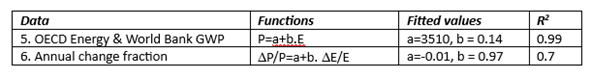
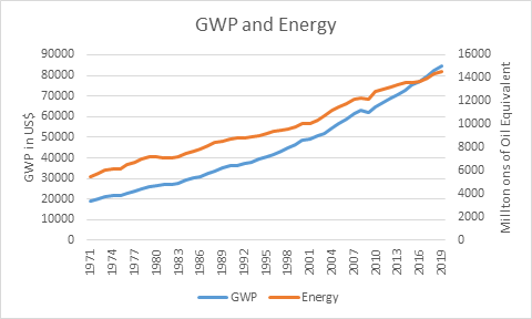
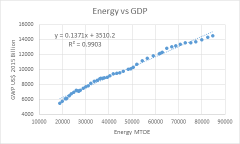
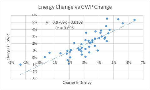
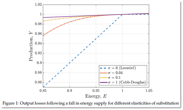
is 0.97, rather than the 0.03-0.04 value assumed by Neoclassical economists. Instead of production being “quite insensitive to energy”, to a reasonable first approximation, production is Energy.

Table 3 shows the coefficients for regressing GDP and change in GDP |(Y/Y) against linear equations for Energy and change in Energy (E/E).

Table 3: Regression of Energy against Gross World Product

Figure 1: Gross World Product and Energy Consumption over time

Figure 2: Energy vs GWP

Figure 3: Ratio of GWP in US$2015 billion to Energy in MTOE from 1971 till 2019

Figure 4: Change in GWP and Change in Energy in Percent p.a.


Figure 5: Correlation of change in Energy and change in GWP in Percent p.a.

This empirical data, as Bachmann et al. unintentionally show, is an effective refutation of the Neoclassical theories of production and income distribution, and confirmation of the Post-Keynesian theories.

They compare the polar opposites of the Cobb-Douglas and the Leontief in a CES production function, where the elasticity of substitution between inputs for Cobb-Douglas equals 1 and that for Leontief equals 0. They correctly lay out the implications of the Leontief case, that:

Leontief production… implies that Y = E/ … and hence logY = log E … Therefore, if the elasticity of substitution is exactly zero, production Y drops one-for-one with energy supply E … Intuitively, the Leontief assumption means that energy is an extreme bottleneck in production: when energy supply falls by 10%, the same fraction 10% of the other factors of production X lose all their value (their marginal product drops to zero) and hence production Y falls by 10%. (Bachmann et al. 2022, Appendix, pp. 5-6. Emphasis added)

They plotted the theoretical relationships between energy input and GDP output for different values of the substitution parameter in their Figure 1 (reproduced as Figure 6 here).

Figure 6: Bachmann et al.’s theoretical predictions of change in output for a change in energy

They then rejected the Leontief function, on the grounds that its prediction of a 1:1 fall in production for a fall in energy leads to nonsensical results in terms of Neoclassical theory:

Extreme scenarios with low elasticities of substitution and why Leontief production
at the macro level is nonsensical
… The blue dashed line in Figure 1 showed that output falls one-for-one with energy supply in the Leontief case… the marginal product of energy jumps to 1/ [their exponent for energy] while the marginal product of other factors … falls to zero. If … factor prices equal marginal products, this then implies that similarly the price of energy jumps to 1/ and the prices of other factors a fall to zero… this then also implies that the expenditure share on energy jumps to 100% whereas the expenditure share on other factors falls to 0%. We consider these predictions to be economically nonsensical. (Bachmann et al. 2022, p. 15. Italicised emphasis added)

These predictions are nonsensical, but at the same time, the Leontief case fits the empirical data (which, following Solow’s lead, they did not consult). It is not the data which is false, but the assumption they made that “factor prices equal marginal products”. Therefore, wages, profits and the price of energy cannot be based upon the “marginal product” of labour, capital and energy respectively. The Neoclassical Cobb-Douglas model of production is false, and the Post-Keynesian Leontief model of production is correct. The question now remains as to why the Leontief model is correct.

From Empirical Regularity to the Role of Energy in Production

The Leontief Production Function began as an empirical regularity between GDP, however measured, and Capital, however measured. The ratio was relatively constant over time and showed no trend—see Figure 7 for Capital to Output ratios derived from the Penn World Tables database.

Figure 7: Capital to Output Ratios are reasonably constant over time

This led to the pragmatic Post-Keynesian school adopting the capital to output ratio as its “production function”, with the justification that this relationship was found in the data, but with no real explanation as to why it was found. Leaving aside the minimum form in which the LPF is often expressed but seldom used, we have, as in the Goodwin model (Goodwin 1967):


Here v is the capital to output ratio. With K having the dimension of Widgets, and Y of Widgets per year, for dimensional accuracy, v must be a time constant denominated in Years.

The empirical regularity behind the LPF can be explained by the aphorism that Ayres, Standish and I applied in “A Note on the Role of Energy in Production” (Keen, Ayres, and Standish 2019), that:

labour without energy is a corpse, while capital without energy is a sculpture. (Keen, Ayres, and Standish 2019):

This suggested that the inputs of Labour and Capital assumed by both the CDPF and the LPF should be replaced by the energy inputs to both Labour and Capital, via the substitution shown in Equation :


Here respectively L and K stand for units of Labour and Capital, EL and EK represent the energy consumed by a unit of Labour and a unit of Capital, and eL and eK are time constants (dimensioned by 1/Year) representing the proportion of these inputs that are turned into useful work over a Year. This then suggests a way to derive the LPF from the dimensionality of the substitution proposed in Equation (5). In the standard single commodity CDPF and LPF, Y and K are denominated in “widgets per year” and “widgets” respectively—units of a universal commodity that can be used for either investment or consumption:


The substitution in (5) on the other hand has the dimensionality of units of Energy per year:


Call this Q, denominated in units of Energy per year, to distinguish it from Y, denominated in units of widgets per year:


Y is therefore equal to Q divided by EK:


Equating Equation (9) with Equation (4) shows that the empirically derived capital to output ratio v is in fact the inverse of the proportion of inputted energy that machinery turns into useful work:


This provides a physical explanation for the empirical regularity on which the Post-Keynesian model of production is based: it is due to the role of machinery in turning energy—predominantly fossil fuel energy—into useful work. This model therefore ties Post-Keynesian theory to the initial accurate insights of the Physiocrats, that Nature is the source of wealth, and that what human ingenuity does is enable the conversion of “this superfluity that nature accords him as a pure gift” (Turgot 1774, p. 9) into useful work. Given the close relationship between GDP and Energy shown in Figure 2 to Figure 5, at a first approximation, GDP is useful energy. Equation (9) can therefore be used in place of Equation (4) in Post-Keynesian models.

The Post-Keynesian model is also consistent with the Laws of Thermodynamics, including the Second Law (which the Physiocrats did not realise) that doing work generates waste as well as desired output. With the capital to output ratio averaging 4 globally, and ranging between 3 and 5 for developed nations, the magnitude of eK is of the order of 0.2-0.33. This then quantifies the waste generated in production as being of the order of 0.67-0.8: humanity generates more waste than output. The constancy of the capital to output ratio, much criticised by Neoclassical economists, is in fact due to the impossibility of substituting any other input for energy, and intrinsic limits to the efficiency of conversion of energy into useful work given by the Second Law of Thermodynamics.

Conclusion

The Neoclassical Cobb-Douglas Production Function, with its exponents assumed to be equal to the income shares of factor inputs, and also equal to the marginal product of those inputs, cannot be reconciled with energy data, or with the Laws of Thermodynamics, and it is therefore wrong.

The Post-Keynesian Leontief Production Function, on the other hand, is not only empirically accurate, but is also consistent with the Laws of Thermodynamics. Though the construction of a universal commodity in aggregate production functions has always been a convenience, the fact that GDP and Energy are so tightly coupled means that the LPF is a reasonable first approximation to reality. Solow’s observation that “As long as we insist on practicing macroeconomics we shall need aggregate relationships” (Solow 1957, p. 213) is correct, but the only aggregate production function that fits the bill is the Leontief Production Function.


Bachmann, Rüdiger, David Baqaee, Christian Bayer, Moritz Kuhn, Andreas Löschel, Benjamin Moll, Andreas Peichl, Karen Pittel, and Moritz Schularick. 2022. ‘Was wäre, wenn…? Die wirtschaftlichen Auswirkungen eines Importstopps russischer Energie auf Deutschland; What if? The macroeconomic and distributional effects for Germany of a stop of energy imports from Russia’, ifo Schnelldienst, 75.

Cantillon, Richard. 1755. Essay on Economic Theory (Ludwig von Mises Institute).

Cobb, Charles W., and Paul H. Douglas. 1928. ‘A Theory of Production’, The American Economic Review, 18: 139-65.

Eddington, Arthur Stanley. 1928. The Nature Of The Physical World (Cambridge University Press: Cambridge).

Engström, Gustav, and Johan Gars. 2016. ‘Climatic Tipping Points and Optimal Fossil-Fuel Use’, Environmental and Resource Economics, 65: 541-71.

Feenstra, Robert C., Robert Inklaar, and Marcel P. Timmer. 2015. ‘The Next Generation of the Penn World Table’, American Economic Review, 105: 3150-82.

Felipe, J., and J. S. L. McCombie. 2014. ‘The Aggregate Production Function: ‘Not Even Wrong”, Review of Political Economy, 26: 60-84.

Felipe, Jesus, and John McCombie. 2011. ‘On Herbert Simon’s criticisms of the Cobb-Douglas and the CES production functions’, Journal of Post Keynesian Economics, 34: 275-94.

———. 2020. ‘The illusions of calculating total factor productivity and testing growth models: from Cobb-Douglas to Solow and Romer’, Journal of Post Keynesian Economics, 43: 470-513.

Felipe, Jesus, and John S. L. McCombie. 2007. ‘Is a Theory of Total Factor Productivity Really Needed?’, Metroeconomica, 58: 195-229.

Fisher, Franklin M. 1971. ‘Aggregate Production Functions and the Explanation of Wages: A Simulation Experiment’, The Review of Economics and Statistics, 53: 305.

Georgescu-Roegen, Nicholas. 1993. ‘Thermodynamics and We, the Humans.’ in J. C. Dragan, E. K. Seifert and M. C. Demetrescu (eds.), Entropy and bioeconomics: Proceedings of the First International Conference of the European Association for Bioeconomic Studies, Rome 28-30, November 1991 (Nagard: Milan).

Goodwin, Richard M. 1967. ‘A growth cycle.’ in C. H. Feinstein (ed.), Socialism, Capitalism and Economic Growth (Cambridge University Press: Cambridge).

Harcourt, G. C. 1972. Some Cambridge Controversies in the Theory of Capital (Cambridge University Press: Cambridge).

Keen, Steve, Robert U. Ayres, and Russell Standish. 2019. ‘A Note on the Role of Energy in Production’, Ecological Economics, 157: 40-46.

Marshall, Alfred. 1890 [1920]. Principles of Economics ( Library of Economics and Liberty).

McCombie, John S. L. 2000. ‘The Solow Residual, Technical Change, and Aggregate Production Functions’, Journal of Post Keynesian Economics, 23: 267-97.

———. 2001. ‘Reflections on Economic Paradigms and Controversies in Economics’, Zagreb International Review of Economics and Business, 4: 1-25.

Samuelson, Paul A. 1979. ‘Paul Douglas’s Measurement of Production Functions and Marginal Productivities’, Journal of Political Economy, 87: 923-39.

Shaikh, Anwar. 1974. ‘Laws of Production and Laws of Algebra: The Humbug Production Function’, Review of Economics and Statistics, 56: 115-20.

———. 1980. ‘Laws of production and laws of algebra: Humbug II.’ in Edward J. Nell (ed.), Growth, Profits and Property (Cambridge University Press).

———. 1987. ‘Humbug production function.’ in John Eatwell, Murray Milgate and Peter Newman (eds.), The New Palgrave: A Dictionary of Economics (Palgrave Macmillan).

———. 2005. ‘Nonlinear Dynamics and Pseudo-Production Functions’, Eastern Economic Journal, 31: 447-66.

Smith, Adam. 1776. An Inquiry Into the Nature and Causes of the Wealth of Nations (Liberty Fund: Indianapolis).

Solow, R. M. 1974a. ‘Intergenerational Equity and Exhaustible Resources’, Review of Economic Studies, 41: 29.

Solow, Robert M. 1957. ‘Technical Change and the Aggregate Production Function’, The Review of Economics and Statistics, 39: 312-20.

———. 1974b. ‘The Economics of Resources or the Resources of Economics’, The American Economic Review, 64: 1-14.

Stiglitz, Joseph. 1974a. ‘Growth with Exhaustible Natural Resources: Efficient and Optimal Growth Paths’, The Review of Economic Studies, 41: 123-37.

Stiglitz, Joseph E. 1974b. ‘Growth with Exhaustible Natural Resources: The Competitive Economy’, Review of Economic Studies, 41: 139.

Turgot, Anne Robert Jacques. 1774. Reflections on the Formation and Distribution of Wealth (London: Spragg).

Ulgiati, Sergio, and Carlo Bianciardi. 2004. ‘Thermodynamics, Laws of.’ in J. Cleveland Editor-in-Chief:   Cutler (ed.), Encyclopedia of Energy (Elsevier: New York).


It’s a Mixed Credit-Fiat World

In contrast to its attitude to private debt, which it ignores, mainstream economics obsesses about government debt. But this volte-face doesn’t besmirch its record of being 100% wrong.

This is the first half of chapter nine of my draft book Rebuilding Economics from the Top Down, which will be published later this year by the Budapest Centre for Long-Term Sustainability

The previous chapter was Why Credit Money Matters, which is published here on Patreon and here on Substack.
If you like my work, please consider becoming a paid subscriber from as little as $10 a year on Patreon, or $5 a month on Substack

Government debt, mainstream economics tells us, is a scourge to be minimized, if it can’t be entirely avoided. These quotes are from Mankiw’s influential macroeconomics textbook {Mankiw, 2016 #6107}, with indicative passages highlighted:

When a government spends more than it collects in taxes, it has a budget deficit, which it finances by borrowing from the private sector or from foreign governments. The accumulation of past borrowing is the government debt… (555)

The government debt expressed as a percentage of GDP roughly doubled from 25 percent in 1980 to 47 percent in 1995. The United States had never before experienced such a large increase in government debt during a period of peace and prosperity. Many economists have criticized this increase in government debt as imposing an unjustifiable burden on future generations… (557)

These trends led to a significant event in August 2011: Standard & Poor‘s, a major private agency that evaluates the safety of bonds, reduced its credit rating on U.S. government debt to one notch below the top AAA grade. For many years, U.S. government debt was considered the safest around. That is, buyers of these bonds could be completely confident that they would be repaid in full when the bond matured. Standard & Poor’s, however, was sufficiently concerned about recent fiscal policy that it raised the possibility that the U.S. government might someday default. (559)

Increases in government debt are a concern because they place a burden on future generations of taxpayers and call into question the government’s own solvency. (595)

This attitude towards government debt and deficits—that government debt should be minimised, that deficits are undesirable, that interest payments on government debt are a punitive impost on future generations, and that high debt and high interest payments can even lead to a government going bankrupt—are key facets of contemporary politics. They were behind the attempt by the UK Cameron government to run surpluses rather than deficits, on the principle that, by “saving for a rainy day”, the government would have more money on hand when crises struck in the future. They lie behind the recurring “debt ceiling” debates in the US Congress. They are the basis of the Eurozone rules, enshrined in the Maastricht Treaty, that government debt should not exceed 60% of GDP, and deficits should be no more than 3% of GDP.

And they are all completely wrong, as is easily shown by looking at the accounting of the mixed credit-fiat monetary system in which we live. I will explain this very, very slowly. It may be tedious to read—it was tedious to write!—but this is necessary, given that utterly fallacious beliefs about the financial system are ingrained into, and damage, our political and social systems, thanks to erroneous mainstream economic thinking.

  1. The Fundamentals of Fiat Money Creation

Figure 30 shows the absolute basic accounting for a Credit money system: banks create money by marking up both sides of their balance sheets. They add Credit dollars per year to Deposits, which are their Liabilities; and they add precisely the same sum to Loans, which are their Assets.

For the non-bank private sector, the act of borrowing also increases its Assets and Liabilities equally: Deposits, which are its Assets, rise by Credit dollars per year, and Loans, which are its Liabilities, rise by precisely the same amount. There is therefore no change in the net worth of either the Banking Sector, or the Non-Bank Private Sector from the creation of credit-money.

Figure 30: The fundamental accounting for Credit Money

The Government’s role in money creation can be considered the same way, by modelling the two fundamental actions of governments: spending on the non-government private sector (either in the form of purchases or transfers), and taxation of the private sector. Figure 31 adds these to the Non-Bank Private Sector’s Godley Table in Figure 30, but without completing the double-entry.

Figure 31: Introducing Government Spending and Taxation without completing the double-entry

How should it be completed? I hope that it is obvious that the only way to complete this double-entry picture is that government spending increases the Equity—the net financial worth—of the non-bank private sector, while taxation reduces it.

This is shown in Figure 32. Government spending increases the net financial worth—the difference between financial assets and financial liabilities—of the private sector, and taxation reduces it.

Figure 32: The double-entry view of Government Spending and Taxation

Figure 33 adds the Banking Sector’s Godley Table to the model, but also without completing the double-entry.

Figure 33: Government Spending and Taxation including the Banking Sector without completing the double-entry

The only sensible way to complete this picture is to add an Asset which is increased by government spending (and reduced by taxation)—and this Asset is normally called “Reserves”. That is done in Figure 34, which shows that government spending increases Reserves and Taxation reduces them.


Figure 34: Government Spending increases Reserves as well as Deposits—and taxation reduces them

At this point, several things should be obvious. Firstly, from the Liabilities side of the Banking system’s ledger, government spending creates money in the same way that new bank loans do, by increasing the Deposit accounts of the non-bank private sector. Similarly, taxation destroys money in the same way that the repayment of bank loans does, by reducing the Deposit accounts of the non-bank private sector.

Secondly, from the Assets side, net government spending—when government spending exceeds taxation—also increases the Assets of the banking sector, in the form of Reserves. This again is akin to how net loan growth—when new loans exceed the repayment of old loans—increases the Assets of the banking sector, in the form of Loans.

We can simplify the exposition of government money creation by defining the difference between government spending and taxation as the Deficit, and using that in future tables rather than using two rows for government spending and taxation respectively:


It follows therefore that a government Deficit—an excess of government spending over taxation—creates money for the Non-bank Private Sector, and creates Reserves for the Banking Sector, as shown in Figure 35.

Thirdly, since a Deficit adds to the Assets of the Non-bank Private Sector, without creating an offsetting Liability, as is the case with a bank loan, a Deficit increases the net worth—the Equity—of the Non-Bank Private Sector. Far from borrowing money from the private sector, as Neoclassical economists claim, the Deficit creates both money and net financial worth for the private sector.

Figure 35: A Government Deficit increases the net financial worth of the private sector

This is already a dramatically different assertion to the conventional wisdom that, as Mankiw puts it, a budget deficit is financed “by borrowing from the private sector” {Mankiw, 2016 #6107, p. 555}. And unlike the conventional wisdom, this assertion is logically sound. The only way the conventional wisdom could be correct would be if the Deficit had a negative impact on Deposit accounts. Then borrowing would occur as Deposits fell, another Asset of the non-bank private sector—”Loans to the Government”—rose. But in that case, government spending would have to decrease Deposits, and taxation would have to increase them! The conventional wisdom of economics, as is so often the case, is absurdly false.

Instead, just as bank lending creates money by increasing the banking sector’s Assets (Loans) and Liabilities (Deposits) simultaneously, a government deficit creates money by increasing the banking sector’s Assets (Reserves) and Liabilities (Deposits) simultaneously.

This leads to a general principle for money creation: since money is predominantly the Deposit accounts of the Non-Bank Private Sector, to create money, a financial operation must increase both the Assets and the Liabilities of the Banking Sector.

For banks, the process is easy—and this is why banks offer Deposit accounts in the first place. When a bank creates a loan, it marks up both sides of its balance sheet: it increases its Assets by adding to Loans, and it increases its Liabilities by adding to its customer Deposits. This is not possible for a Non-Bank Financial Institution: it can reallocate funds between its Assets, and gain when Assets increase in value, but it can’t increase the value of its Assets by its own operations. Banks can—so long as they can find willing borrowers.

The process of government money creation is more complicated than that of credit money creation, because the government can’t directly write up bank Assets and Liabilities. Instead, it has to increase a bank Asset—Reserves—after which banks will then allocate the same sums to the Deposit accounts of their customers.

How are Reserves increased? To show that, we need to introduce a third Godley Table, that of the Central Bank. That is done in Figure 36, but without completing the double-entry logic.

Figure 36: Introducing the Central Bank without completing the double-entry

How do we balance that row? We could show this as negative equity for the Central Bank—if, as is the practice amongst many advocates of MMT (Modern Monetary Theory), we consolidated the Central Bank and the Treasury into one entity. But there’s no need to make that simplification with Minsky. We can, instead, show the financial sector in its realistic complexity, by adding another Liability of the Central Bank—the “deposit account” of the Treasury at the Central Bank. This is called the “Consolidated Revenue Fund” (CRF) in the UK, and the “Treasury General Account” in the USA (TGA). I use the American acronym in Figure 37.

Figure 37: The Central Bank with double-entry completed and the Treasury TGA introduced

Reserves rise because of a transfer of funds from the TGA to Reserves. To show how these funds are generated, we need to add the Treasury’s Godley Table. That is done in Figure 38, again without completing the double-entry.

Figure 38: The Treasury Table introduced, without completing the double-entry

I hope it’s obvious that the only way to balance this line is the make the second entry in the Treasury’s Equity. That is done in Figure 39, which shows that the Treasury’s position is the exact opposite of the Non-Bank Private Sector’s: the positive Equity that the Deficit generates for the Private Sector is created by the Treasury going into identical negative Equity.

Figure 39: The completed basic picture of Government money creation

This simple picture appears unnatural to many people on first sight: what is the government doing, going into negative equity? Isn’t that a bad thing?

In fact, the government being in negative financial equity is the essence of fiat money. Banks create credit money by expanding their Assets and Liabilities equally; this results in a matching expansion of the non-bank private sector’s Liabilities and Assets. Governments create fiat money by going into negative Equity, which creates matching positive Equity for the non-bank private sector.

This can only work in the places in which a government’s liabilities are accepted as money, which define the locations in which it is the government. This is especially so for government operations on bank accounts. Sometimes, one country’s notes and coins are accepted as means of payment in another—you can sometimes use Euros to buy goods in Hungary, for example. But only the Hungarian government can directly add to Hungarian bank accounts by putting more Forints into them via government spending than it debits from them via taxation.

It is also of the essence of financial assets—claims on other entities—that the sum of all financial assets is zero. If one entity is in positive financial equity, then all other entities in an economy as in precisely the same negative financial equity with respect to it. What entity can sustain permanent negative financial equity? Not banks, because, by definition, banks must be in positive financial equity: a bank whose liquid liabilities exceed its liquid assets is bankrupt. The non-bank private sector can sustain negative financial equity, if its income is sufficient to service its debts, but it’s not a comfortable situation for individuals or companies to have liabilities that exceed their assets.

But a government, whose liabilities are money in its country, can always service its net negative financial position because it creates its own money. Finally, fiat money is backed by the extensive nonfinancial assets of a government: the unalienated land, the buildings, infrastructure, military, etc., of a nation state. There is, in other words, no problem with a government being in negative financial equity with respect to its own currency. It also means that, by running a sufficiently large deficit, it can ensure that both the Banking Sector and the Non-Bank Private Sector are in positive equity.

At this absolutely fundamental level then, net government spending does not involve borrowing from the private sector, and in fact it creates fiat money for the private sector. But what about government bonds? How do they change the picture? Don’t they mean that the government is borrowing from the private sector?

  1. Government Bond Sales

One obvious consequence of the fundamental situation outlined above is that the Treasury’s account at the Central Bank must go negative. In and of itself, this isn’t a problem, since the Treasury and the Central Bank are both wings of the government, and in terms of where the Central Bank’s income is remitted, the Treasury is the effective owner of the Central Bank. It also has no implications for the solvency of the Central Bank, since the negative value of the TGA is precisely offset by the positive value of Reserves. Finally, as Central Banks themselves acknowledge {Bholat, 2016 #6037}, unlike a private bank, it is not necessary for a Central Bank to be in positive equity.

However, virtually all governments have passed laws requiring the TGA to not go negative—and this is the real function of Treasury Bond sales. The upshot of these laws is that Treasuries are required to sell bonds equivalent in value to the deficit, plus interest on existing bonds.

I’ll introduce government bond sales in the simplest possible way—as a sale of a bond to the Central Bank. This is in fact illegal in most countries, since they have also enacted laws that forbid the Central Bank from buying Bonds directly from the Treasury. But there is absolutely no practical impediment to this operation. It also has the side effect that interest payments are unnecessary: in most countries, the Treasury doesn’t pay interest on bonds owned by the Central Bank, and in those which do, the interest income is remitted back to the Treasury anyway. Therefore, interest payments on bonds—the cause of much angst in mainstream economics—can be omitted from the model.

This hypothetical situation is shown in Figure 40. If the value of bonds sold by the Treasury to the Central Bank—shown as the flow —was equal to the Deficit, then the TGA would remain positive (or at least non-negative). This makes no practical difference to fiat money creation—that relies solely upon the Treasury going into negative equity—but is an aesthetic improvement on the situation shown in Figure 39, in that both Liability accounts of the Central Bank (Reserves and the TGA) would be positive. The Central Bank also has positive Assets, whereas in Figure 39 they are zero.

Figure 40: Treasury Bond Sales Direct to the Central Bank

The upshot of this arrangement for the Banking Sector is that the Asset that Deficits generate for it—Reserves—don’t normally earn income (by “normally” I mean “before the “Global Financial Crisis”). I suspect this detail—and not any desire to force prudence upon government money creation—is why most countries have made direct purchases of Treasury Bonds by the Central Bank illegal. Instead, these laws require the Treasury to sell Bonds to the private banks (and primary dealers), with the Central Bank then able to buy bonds from private banks in the “secondary market”.

The “magic” of this arrangement for the Banks is that the funds that private banks use to buy Bonds are created by the deficit itself—both the current deficit and the accumulation of past deficits known as government debt. Banks swap non-income-earning and non-tradeable Reserves for income-earning and tradeable Treasury Bonds. Since the Treasury does have to pay interest on bonds owned by the non-government sector, the act of selling Bonds to the Private Banks also necessitates paying interest on existing Bonds—which is otherwise known as existing Government debt. This generates an income stream for the Banking Sector.

Figure 41 shows this legally required situation, without completing the double-entry details for the impact of interest on bonds for Private Banks. It should be obvious that this payment of interest adds to the net worth of the Banking Sector. And, just as the positive equity from the deficit for the non-bank private sector is created by the Treasury going into negative equity, the positive equity for the Banking Sector from government interest payments is also created by the Treasury going into negative equity.

Figure 41: Bond Sales to Private Banks, without completing the double-entry

A comparison of Figure 39 to Figure 40 and Figure 41 shows how absurd it is to describe the Treasury selling Bonds to the Banking Sector as the Treasury borrowing from the Banking Sector.

Neither arrangement is needed for the Treasury to create fiat money: the deficit alone does that, as Figure 39 shows, and it is financed by the Treasury going into negative equity, not by it selling Bonds to anyone. The only thing preventing Figure 39 from being the normal situation is a law requiring the TGA to not go into overdraft; if that law were repealed, there would be no need for Bond sales at all. Similarly, the only thing preventing Figure 40—direct Treasury bond sales to the Central Bank—is a law prohibiting it. These laws benefit the Banking Sector by letting it earn interest income on the Asset created for it by the Treasury, rather than (normally) not earning interest on Reserves.

Figure 42 completes the picture by showing interest on bonds as increasing the Equity of the Banks. It is then obvious that, just as the deficit creates net equity for the non-bank private sector, the payment of interest on bonds creates net equity for the banking sector.

Figure 42: Treasury Bond sales complicate the process, but don’t change the nature of fiat money

The final operation needed to complete the basic picture of government finances is the sale of Treasury Bonds by Banks to the non-bank private sector. Most of these sales are to Non-Bank Financial Institutions (NBFIs), but for simplicity I simply show this as a sale to the Non-Bank Private Sector in Figure 43. Once again, it would be ridiculous to describe this sale of a financial asset by the Banking Sector to the Non-bank Private Sector as “the government borrowing from the private sector”, but that’s how it’s described by Neoclassical economists.

Figure 43: Bond Sales to Non-Banks by Banks

However, this operation is the only type of Bond sale that affects the quantity of money, and it reduces it rather than increasing it: Deposit accounts at banks fall, while the Non-bank Private Sector’s holdings of an income-earning Asset rise. The sale of Treasury Bonds by Banks to the Non-bank Private Sector—mainly to Non-Bank Financial Institutions (NBFIs)—thus destroys money.

We can now combine this model of fiat money creation—for that is what a Deficit actually is—with the model of credit money creation outlined in the previous chapter to show the real-world consequences of misunderstanding money creation. There is no better indication of the negative impact of mainstream misunderstandings about money than its role in causing the Great Depression.

Puncturing the Hubris of Economics

The greatest disjuncture in the social sciences is between the image that economists have of their discipline, and its reality. A decade before David Graeber published Debt: the First 5000 Years (Graeber 2011), the future chief economic advisor to President George W. Bush published a paper with the confronting title of “Economic Imperialism” (Lazear 2000), in the discipline’s most prestigious journal, The Quarterly Journal of Economics. Lazear was not criticizing economics for attempting to take over other fields of social science, but lauding it for doing so:

There are two claims made in this essay. The first is that economics has been imperialistic, and the second is that economic imperialism has been successful. (p. 103)

This article is valuable, not for its insights, but for highlighting the rampant hubris of mainstream “Neoclassical” economics at the apogee of its influence. It opened with the declaration that “Economics is not only a social science, it is a genuine science” (p. 99). More than 40 pages and over 17,000 words later, it closed with:

Economics has been successful because, above all, economics is a science. The discipline emphasizes rational behavior, maximization, trade-offs, and substitution, and insists on models that result in equilibrium. Economists are pushed to further inquiry because they understand the concept of efficiency. Inefficient equilibria beg for explanation and suggest that there may be gaps in the underlying models that created them.

Because economics focuses so intently on maximization, equilibrium, and efficiency, the field has derived many implications that are testable, refutable, and frequently supported by the data. The goal of economic theory is to unify thought and to provide a language that can be used to understand a variety of social phenomena. The most successful economic imperialists have used the theory to shed light on questions that lie far outside those considered traditional. The fact that there have been so many successful efforts in so many different directions attests to the power of economics. (p. 142)

The paper’s length gives the clue that this was a solicited paper, intended to provide an assessment of the state of economics at the beginning of the new millennium:

To commemorate the end of one century and the beginning of another, the Board of Editors of the Quarterly Journal of Economics invited a select group of distinguished economists to submit articles assessing the accomplishments of the discipline of economics in the twentieth century. We have asked each of these scholars to reflect on “what we know that Marshall did not” in different areas of economics. (Editors 2000)

If ever a discipline deserved to be skewered, economics at the turn of the millennium was it, and David Graeber wielded the skewer with aplomb and humour. Economics is not a science, but a collection of self-referential and self-supporting myths, each of which cannot be dislodged without causing the entire edifice to collapse. Debt: The First 5,000 Years focused upon the myth that money sprung out of barter, and its attendant myth that the State and the Market are “diametrically opposed principles”, when in fact “they were born together and have always been intertwined”.

The evidence—the sort of thing on which a genuine science is based—that a society based upon barter has never existed is overwhelming. As David put it:

The story of money for economists always begins with a fantasy world of barter…

For centuries now, explorers have been trying to find this fabled land of barter—none with success…

missionaries, adventurers, and colonial administrators were fanning out across the world, many bringing copies of Smith’s book with them, expecting to find the land of barter. None ever did. They discovered an almost endless variety of economic systems. But to this day, no one has been able to locate a part of the world where the ordinary mode of economic transaction between neighbors takes the form of “I’ll give you twenty chickens for that cow.”

I never expected David’s well-documented evidence that barter-based societies were mythical to convince Neoclassical economists to abandon the myth, because without that myth, their entire paradigm unravels. But David’s work did strengthen the resolve of, and improve the analysis done by, the subsets of critical economists to which I belong: the Post-Keynesians, the Evolutionary Economists, the Biophysical Economists, and Modern Monetary Theorists. We frequently find ourselves referring to David’s work when we attack the myth of barter, and his work has also had a creative impact upon us.

In my case, David’s explanation of the origins of money in credit directly influenced my modelling the role of credit in economics. Building on David’s work, as well as that of radical economists like Joseph Schumpeter (Schumpeter 1934) Irving Fisher (Fisher 1933), Hyman Minsky (Minsky 1963; Minsky 1977, 1982), Basil Moore (Moore 1979), Augusto Graziani (Graziani 2003, 1989), and Wynne Godley (Godley 1999; Godley and Lavoie 2005), my colleagues Michael Hudson (Hudson 2009, 2004, 2020, 2024) Dirk Bezemer (Bezemer 2014; Bezemer 2011, 2010), Gael Giraud (Keen and Giraud 2016), Matheus Grasselli (Giraud and Grasselli 2019; Costa Lima et al. 2014; Grasselli and Costa Lima 2012) and I (Keen 2023; Keen 2021, 2015) have shown that credit plays an essential role in economics.

But neither our work, nor David’s, has influenced mainstream economics one jot. The last resort of the Neoclassical scoundrel is the argument that the fact that money didn’t evolve out of barter, but out of credit, is irrelevant: credit makes no significant difference to macroeconomics. Therefore, it’s easier to stick with the myth, and model capitalism as a barter system. Nothing of significance is lost.

This is how Neoclassical economists initially reacted to the Bank of England‘s startling admission in 2014 that the non-mainstream economists who asserted that bank lending—otherwise known as credit—created money, were correct, and the mainstream was wrong, in the paper “Money creation in the modern economy”:

The reality of how money is created today differs from the description found in some economics textbooks: Rather than banks receiving deposits when households save and then lending them out, bank lending creates deposits. (McLeay, Radia, and Thomas 2014, p. 14. Emphasis added)

You might think that, though economists could ignore one troublesome anthropologist, surely, they couldn’t ignore the Bank of England? I did too initially, but time proved me wrong.

Firstly, they disputed that the fact that bank lending creates money actually matters:

We establish a benchmark result for the relationship between the loanable-funds and the money-creation approach to banking. In particular, we show that both processes yield the same allocations when there is no uncertainty. In such cases, using the much simpler loanable-funds approach as a shortcut does not imply any loss of generality. (Faure and Gersbach 2022, p. 107; Faure and Gersbach 2017. Emphasis added)

Only a Neoclassical economist could write “when there is no uncertainty” and “does not imply any loss of generality” in the same paragraph…

Finally, they ignored the Bank of England completely.
When the Swedish Central Bank awarded its fake “Nobel” in Economics (Offer and Söderberg 2016) to Ben Bernanke, for a model of banking in which bank loans don’t create money, the so-called “Scientific Background” paper for his Prize did not even cite the Bank of England‘s contrary declaration about bank lending (Committee for the Prize in Economic Sciences in Memory of Alfred Nobel 2022).

David’s name was, of course, nowhere to be seen.

It would be futile, therefore, to expect economics to reform itself because of David’s exposé of the myth of barter. Instead, we should focus on David’s other gifts: the capacity to develop a realistic framework for understanding the world—such as his concept of “bullshit jobs” (Graeber 2018)— and to whimsically ridicule the absurd in the process.

The concept of “Bullshit Jobs” made intuitive sense to normal people, many of whom provided the materials for that book. But according to the Neoclassical theory that wages are based upon a worker’s “marginal product”, bullshit jobs could not exist, because the “marginal product” of a bullshit job is negative.

So then, how can we make sense of this obviously real phenomenon? Blair Fix argues, based on an empirically derived and supported hypothesis, that incomes are based not on the productivity of the individual, but on their rank in a hierarchy:

Neoclassical economists argue that the rich are different, because they are more productive… Marxists, in contrast, argue that the rich are different, because they exploit workers… What makes the rich different, I propose, is… their greater control of subordinates—what I call ‘hierarchical power’. (Fix 2020, p. 2)

This generates an incentive for the creation of bullshit jobs within a corporation, since the more people who report to a manager, the higher that manager’s status, and rank in a corporate hierarchy, will be. Bullshit jobs have nothing to do with productivity, and everything to do with power.

Similarly, I have developed a framework to show that credit is a critical aspect of a capitalist economy, by turning what Neoclassical economists think is their strength—mathematics—against them. Chronologically, this was done firstly by finding overwhelming empirical evidence that credit does matter; secondly, by developing a computer program—named after another great iconoclast, Hyman Minsky (Minsky 1982)—which enables a monetary economy to be modelled easily; and thirdly, by developing a mathematical proof that credit is indeed a fundamental determinant of economic activity.

I detail these here to show that key ripostes that economists make to many criticisms—that they lack empirical verification, that they cannot be modelled, and that they cannot be proved—are false. One has to be deliberately blind to the data to not see the impact of credit on the economy, credit can be modelled, but not within the Neoclassical paradigm—one must renounce it instead—and the logical proof that credit matters is irrefutable. This is why Neoclassical economists are so resistant to the well-founded wisdom in David’s work: admit David, and they have to exit themselves.

Credit: The Data

In rejecting Irving Fisher’s argument that the Great Depression was caused by a “debt-deflation”, Bernanke put “the counterargument”:

that debt-deflation represented no more than a redistribution from one group (debtors) to another (creditors). Absent implausibly large differences in marginal spending propensities among the groups, it was suggested, pure redistributions should have no significant macroeconomic effects. (Bernanke 2000, p. 24. Emphasis added)

Apart from the mischaracterisation of credit as “pure redistributions”, this is an empirical proposition, which could have been easily checked against data that existed when Bernanke made this claim. It was wrong then, and even more obviously today, with modern quarterly data on debt from the Bank of International Settlements (Dembiermont, Drehmann, and Muksakunratana 2013).

Figure 1 plots private debt from 1947 till 2023, and credit against the unemployment rate from 1981 to 2023, when the private debt level has exceeded 100% of GDP. The negative correlation between credit and unemployment is visually obvious, and in the period between 1990 and 2015—which covers the boom leading up to the 2007 “Global Financial Crisis” and its aftermath—the correlation exceeded -0.9: when credit rises, unemployment falls, and vice versa. Far from having “no significant macroeconomic effects”, credit is possibly the most significant of all of the determinants of macroeconomic performance.

Figure 1 Private Debt, Credit and Unemployment in the USA:

Empirically then, it is obvious that credit does matter. The remaining question is why does it matter? This is answered partially by comparing two models of banking: the Neoclassical model of “Loanable Funds”, in which banks are “mere intermediaries” which do not lend money, and the real-world model I call “Bank Originated Money and Debt”, in which, as the Bank of England says, “bank lending creates deposits”.

Credit: The Model

As the quote from Faure and Gersbach illustrates, in the Neoclassical model of banking, banks are “mere intermediaries” between savers and borrowers: they take in funds from savers and lend them out to borrowers.

Figure 2 is a very simple rendition of this model: Savers and Borrowers have deposit accounts; they spend out of them at different rates, and the sum of their spending is GDP; and Borrowers pay interest to Savers (for simplicity, I have made the Banks neutral in this model).

Figure 2 shows a run of the model in which, starting in Year 10, Savers lending out 25% of their Deposit accounts every year, until such time as debt reaches 170% of GDP—the peak level of actual US private debt during the GFC. Then the control parameter LendRate is reversed, so that Borrowers pay off the equivalent of 25% of Savers’ deposit accounts every year.

The macroeconomic effect of these dramatic changes in Credit are minimal. There is a small effect of growing GDP as borrowers—who spend more rapidly than savers—take on more debt, and a small effect of falling GDP as borrowers repay debt, but it is relatively trivial: GDP rises from $240 per year at zero debt to $260 per year at a private debt level of 170% of GDP, and this is over a simulation time of seventy years. If this was all credit added to the macroeconomic equation, then it would be sensible to ignore it, as Neoclassicals do.

Figure 2: The Neoclassical “Loanable Funds” model of banking

However, that is not the real-world. In the real-world, as the Bank of England declared, banks create money by issuing new loans. Figure 3 captures this, by showing Loans as an Asset of the Banks rather than of Savers. But otherwise, the model is identical to the Loanable Funds model in Figure 2.

However, the economic outcome couldn’t be more different: GDP grows virtually 100-fold over the 30 years of credit growth, and it falls dramatically as credit goes negative for the subsequent years.

Figure 3: The real-world model of “Bank Originated Money and Debt”

The model confirms that Credit matters, as the data itself showed. The next question—that Neoclassicals don’t even want to ask, let alone answer—is why?

Credit: The Proof

As the models indicate, credit has significant macroeconomic effects when bank lending creates money, but virtually no effect when banks are just conduits between savers and borrowers—as Neoclassical economists pretend that they are. The reason for this difference is easily shown using a device I call a Moore Table, in honour of the great pioneer of endogenous money research in economics, Basil Moore (Moore 1979, 1988; Moore 2006). A Moore Table lays out monetary expenditure and income in an economy in terms of expenditure flows between sectors (or people and companies) in the economy. Each row shows the expenditure by a given sector, and the sectors that are the recipients of that expenditure, with expenditure having a negative sign and income having a positive sign. Necessarily therefore, the sum of each row is zero.

Each column shows the net income of each sector. This can be positive (if income exceeds expenditure) or negative (if expenditure exceeds income), but the aggregate must again be zero.

By construction, the negative of the sum of the diagonal elements of the table is aggregate expenditure, and it is identically equal to the sum of the off-diagonal elements, which is aggregate income. In the limit, if every agent in a country were included in the table, then it would measure that country’s GDP.

Figure 4 shows the simplest example, of an economy with money, but no credit or debt of any kind. Instead, there is a fixed stock of money, with each sector spending on the other two sectors.

Figure 4: Aggregate Expenditure and Income with no lending

Unremarkably, both aggregate expenditure and aggregate income are the sum of the flows A to F, as shown by Equation (1):


Figure 5 shows the Neoclassical model of Loanable Funds, and gives the example of the Services sector lending Credit dollars per year to the Household sector, and the Household sector then spending this borrowed money on the Manufacturing sector. The Household sector also has to pay Interest dollars per year to the Services sector, based on the level of outstanding debt. The transfer of money in the loan is shown across the diagonal, because only income-generating transactions are shown across the rows.

This model has Credit reducing the expenditure that the Services sector can do (you can’t spend money that you have lent to someone else), while increasing the spending that the borrower—the Household sector—can do. This additional spending by Households boosts the income of the Manufacturing sector, but it is precisely offset by the lower level of spending by the Services sector on Manufacturing (the flows A to F in this table do not have to be the same as in Figure 4).

This means that the entry for Credit cancels out on both the diagonal (aggregate expenditure) and the off-diagonal (aggregate income), so that Credit is not part of aggregate expenditure or aggregate income in Loanable Funds. Therefore, if Loanable Funds was an accurate description of what banks actually do, Neoclassicals would be correct to ignore credit, as they do in their macroeconomics.

Figure 5: Aggregate Expenditure and Income with Loanable Funds lending

The only effect of including “peer to peer” lending in this model is that Interest payments become part of Aggregate Expenditure and Income—see Equation (2).


Figure 6 shows the real-world situation of bank lending. Credit adds to both the Assets of the banking sector, and its Liabilities—the deposit accounts of the Household sector. In this simple example, Household then spend this additional money on the Manufacturing sector. The logical and practical import of this situation is that Credit appears only once in both aggregate expenditure—the spending by the Household sector—and aggregate income—the income of the Manufacturing sector. Consequently, Credit does not cancel out, as it did for Loanable Funds.

Figure 6: Aggregate Expenditure and Income with Bank Originated Money and Debt lending

Instead, as Equation (3) shows, Credit is part of Aggregate Expenditure and Income. Given how volatile Credit is—as the US data in Figure 1 shows, it went from plus 15% of GDP in 2007 to minus 5% in 2009—it is the causa causans of macroeconomic instability. By ignoring it, Neoclassicals are modelling a system of petty commodity exchange, not real-world capitalism.


Therefore, empirical data and mathematics, the weapons that Neoclassical economists like to wield to intimidate other social sciences, can instead show that their paradigm is based on myths rather than science. Economics could be a radically different—and even useful—social science if it absorbed, rather than deflected, the criticisms that David made of it. But it never will, because the core elements of the Neoclassical paradigm are antithetical to the evolutionary foundations of genuine social sciences like Anthropology and Sociology.

Equilibrium as a Hallmark of Science?

Above all, the component of the Neoclassical paradigm that makes it impossible for it to be a genuine social science is the obsession with modelling the economy as if it is in equilibrium (Kornai 1971), or as if has an innate tendency to return to equilibrium after an “exogenous shock”. That concept, which Lazear thought was the hallmark of a science, is instead the mark of an intellectual dead end.

Ironically, the founders of the Neoclassical school of thought were aware of this. Jevons wrote in 1888 that:

The real condition of industry is one of perpetual motion and change. Commodities are being continually manufactured and exchange and consumed. If we wished to have a complete solution of the problem in all its natural complexity, we should have to treat it as a problem of motion—a problem of dynamics. But it would surely be absurd to attempt the more difficult question when the more easy one is yet so imperfectly within our power. (Jevons 1888, p. 93. Emphasis added)

Likewise, in predicting what their successors in the 20th century would achieve, John Bates Clark wrote in 1898—in an article entitled “The Future of Economic Theory”, which had a very similar genesis to Lazear’s—that:

The great coming development of economic theory is to take place, as I venture to assert, through the statement and the solution of dynamic problems… A static state is imaginary. All actual societies are dynamic; and those that we have principally to study are highly so. Heroically theoretical is the study that creates, in imagination, a static society. (Clark 1898, pp. 2, 9)

At the end of that century, while devotees like Lazear were exultant about their equilibrium-centric analysis, wiser heads were despairing. The mathematician John Blatt acerbically observed in 1983 that:

A baby is expected to first crawl, then walk, before running. But what if a grown-up man is still crawling? At present, the state of our dynamic economics is more akin to a crawl than to a walk, to say nothing of a run. Indeed, some may think that capitalism as a social system may disappear before its dynamics are understood by economists. (Blatt 1983, p. 5)

Blatt’s prescient remark predated the domination of economic modelling by what economists call Dynamic Stochastic General Equilibrium (DSGE) models, and lest an economist tell you that, therefore, this criticism is out of date, here is “Nobel” Prize winner Paul Romer on the topic of those very same models in 2016:

In the last three decades, the methods and conclusions of macroeconomics have deteriorated to the point that much of the work in this area no longer qualifies as scientific research … macroeconomic pseudoscience is undermining the norms of science throughout economics. If so, all of the policy domains that economics touches could lose the accumulation of useful knowledge that characteristic of true science, the greatest human invention. (Romer 2016, Abstract, p. 1)

Why has economics failed so badly? Arnsperger and Varoufakis provide a paradoxical but convincing argument that the very failures of Neoclassical economics are the source of its power. The failure to prove results they expected—driven primarily by the fact that, when put into dynamic form, the equilibria of their models almost always turned out to be unstable (Blatt 1983, Chapter 7, pp. 111-146)—led to arcane assumptions being added to hang onto their Holy Grail of Equilibrium, despite mathematics which proved that their God did not exist. Rather than causing the paradigm to undergo a desperately needed scientific revolution (Kuhn 1970), this led to the concept of equilibrium being turned into a quasi-religious belief about the innate nature of capitalism, using assumptions that are mind-bogglingly stupid.

However, since these stupid assumptions enabled economists, however tenuously, to hang on to the core beliefs of Marshall (Marshall 1890 [1920]), Jevons and Walras (Walras 1954 [1899]) that capitalism was a utility-maximising and cost-minimising system, and since these core beliefs corresponded to the ideological desires of society’s elite, this transformation of equilibrium from an unfortunate modelling compromise (Clark 1898; Jevons 1888) to the hallmark of a science (Lazear 2000) cemented the prestige of economics in the media and in social policy. As Arnsperger and Varoufakis put it:

such failure, instead of weakening neoclassicism, has reinforced its hold over the imagination of both the elites and the public at large. (Arnsperger and Varoufakis 2006, pp. 6-7)

The resultant belief of today’s Neoclassicals—that a discipline which, in Lazear’s words, “insists on models that result in equilibrium” (Lazear 2000, p. 99)—is therefore a science is beautifully kyboshed by one of the most famous models in science, Lorenz’s “Butterfly” model of turbulence in fluid dynamics, which underpins modern meteorology (Lorenz 1963). With just three variables and three parameters, this model has three equilibria, all of which are unstable—see Figure 7. The three equilibria are obvious in the model: they are the point (0,0,0)—with the simulation beginning very nearby at (1,1,1,), after which it is propelled away—and the two “eyes of the mask”. Rather than being where the model “results in equilibrium”, equilibria are where the model will never be.


Figure 7: Lorenz’s “strange attractor” in which all 3 equilibria of this very simple model are unstable

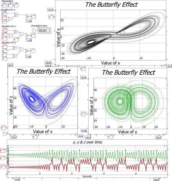
Other pivotal works in post-WWII science show how ignorant economics is of what modern science is. Economics today is obsessed with deriving macroeconomics, the study of the whole economic system, from microeconomics, the assertions (false, of course) that Neoclassical economists make about the behaviour of consumers, firms and markets. Yet over 50 years ago, a real Nobel Prize winner (in Physics), P.W. Anderson, wrote the influential paper “More is Different”, in which he asserted, on the basis of Lorenz’s work and the understanding of complex systems that flowed from it, that what Neoclassicals are attempting to do is impossible. This is because, though reductionism is a valid scientific method (within limits), its obverse of “constructionism” is not:

The main fallacy in this kind of thinking is that the reductionist hypothesis does not by any means imply a “constructionist” one: The ability to reduce everything to simple fundamental laws does not imply the ability to start from those laws and reconstruct the universe… Instead, at each level of complexity entirely new properties appear, and the understanding of the new behaviors requires research which I think is as fundamental in its nature as any other… Psychology is not applied biology, nor is biology applied chemistry. (Anderson 1972, p. 393)

And neither, to continue Anderson’s hierarchy, is anthropology simply applied economics. In fact, a better strategy—in line with David’s method—would be to undertake an anthropological study of economics itself, to work out why this peculiar discipline has simultaneously become both so dominant and so dysfunctional.

Fortunately, there is work—of a fittingly satirical kind—to build upon, in the form of the non-orthodox economist Axel Leijonhufvud’s wonderful parody “Life Among the Econ”:

The Econ tribe occupies a vast territory in the far North. Their land appears bleak and dismal to the outsider, and travelling through it makes for rough sledding; but the Econ, through a long period of adaptation, have learned to wrest a living of sorts from it. They are not without some genuine and sometimes even fierce attachment to their ancestral grounds, and their young are brought up to feel contempt for the softer living in the warmer lands of their neighbours, such as the Polscis and the Sociogs.

Despite a common genetical heritage, relations with these tribes are strained—the distrust and contempt that the average Econ feels for these neighbours being heartily reciprocated by the latter—and social intercourse with them is inhibited by numerous taboos. The extreme clannishness, not to say xenophobia, of the Econ makes life among them difficult and perhaps even somewhat dangerous for the outsider. This probably accounts for the fact that the Econ have so far not been systematically studied. Information about their social structure and ways of life is fragmentary and not well validated. More research on this interesting tribe is badly needed. (Leijonhufvud 1973, p. 327)

In the spirit of David’s whimsical wit, my penultimate conclusion is expressed by correcting the errors in Lazear’s description of economics:

Economics has been successful because, above all, economics is a cult. Its dominant sect emphasizes rational behavior, maximization, trade-offs, and substitution, and insists on models that result in equilibrium, thus insulating itself from 20th century developments in genuine sciences. Economists are pushed to further irrelevance because they are obsessed with the concept of efficiency. Inefficient equilibria beg for dynamics and evolutionary explanations, and I suggest that there may be gaps in the brain wiring of economists who do not understand this.

Because economics focuses so intently on maximization, equilibrium, and efficiency, the field has derived many implications that are untestable, irrefutable, and frequently contradicted by the data. The goal of economic theory is to suppress critical thought and to provide a language that can be used to distort a variety of social phenomena. The most successful economic imperialists have used the theory to shed confusion on questions that lie far outside issues that they deludedly think they comprehend. The fact that there have been so many successful efforts in so many different directions attests to the capacity of economics to deceive.

My ultimate conclusion is a personal one. David began as an influence on my economic thinking when I first read Debt: the First 5000 Years in 2011 while working in Sydney. We became close friends when we met after I moved to London it 2014. That friendship became firmer still when his wife, the love of his life, and intellectual and artistic collaborator Nika Dubrovsky entered the picture.

Figure 8: David, myself, and his wife Nika Dubrovsky, in their home in London in December 2019

I had expected that we’d socialise, bounce ideas off each other, laugh, and collaborate for many years to come. But on September 2nd 2020, those expectations were dashed. Instead, I found myself writing a eulogy to him. It opened, as one does these days, with Tweets:

Oh David! @davidgraeber. . They say only the good die young, but why did you have to be one of them? There’s even more bullshit in the world now that you are no longer with us. It was a pleasure to know you, and it is a tragedy to say goodbye.

I’m an agnostic and so was David @davidgraeber. But if he’s doing anything at all right now, it’s an anthropological study of Heaven. Preceded by a brief study of Hell, but just for comparative reasons. The Devil was sad to see him go.

I’m agnostic, but for the very first time, I am wishing that there is life after death, I told @stacyherbert , when she wrote “He’s actually trending in America now on Twitter! I wonder if he would be mortified by that or laughing his ass off . . . I suspect the latter?”

So yes David, this fellow agnostic wishes he’s wrong, and I hope you can read this and are laughing at what a sentimental twat I’m being. And being jealous of me getting smashed on Tequila as I write this—though I suppose Heaven has much better Tequila than we get down here on the Purgatory that is Earth in 2020.

The only saving grace of David’s far-too-early death is the thought that at least he has missed seeing how much more of a purgatory life on Earth has become in the subsequent years.

Anderson, P. W. 1972. ‘More Is Different: Broken symmetry and the nature of the hierarchical structure of science’, Science, 177: 393-96.

Arnsperger, Christian, and Yanis Varoufakis. 2006. ‘What is neoclassical economics? The three axioms responsible for its theoretical oeuvre, practical irrelevance and, thus, discursive power’, Panoeconomicus, 53: 5-18.

Bernanke, Ben S. 2000. Essays on the Great Depression (Princeton University Press: Princeton).

Bezemer, D. J. 2009. ”No one saw this coming’ – or did they?’, Centre for Economic Policy Research (CEPR). https://voxeu.org/article/no-one-saw-coming-or-did-they.

———. 2014. ‘Schumpeter might be right again: the functional differentiation of credit’, Journal of Evolutionary Economics, 24: 935-50.

Bezemer, Dirk J. 2010. ‘Understanding financial crisis through accounting models’, Accounting, Organizations and Society, 35: 676-88.

———. 2011. ‘The Credit Crisis and Recession as a Paradigm Test’, Journal of Economic Issues, 45: 1-18.

Blatt, John M. 1983. Dynamic economic systems: a post-Keynesian approach (Routledge: New York).

Clark, John Bates. 1898. ‘The Future of Economic Theory’, The Quarterly Journal of Economics, 13: 1-14.

Committee for the Prize in Economic Sciences in Memory of Alfred Nobel, The. 2022. “Financial Intermediation and the Economy.” In. Stockholm: The Royal Swedish Academy of Sciences.

Costa Lima, B., M. R. Grasselli, X. S. Wang, and J. Wu. 2014. ‘Destabilizing a stable crisis: Employment persistence and government intervention in macroeconomics’, Structural Change and Economic Dynamics, 30: 30-51.

Dembiermont, Christian, Mathias Drehmann, and Siriporn Muksakunratana. 2013. ‘How much does the private sector really borrow? A new database for total credit to the private nonfinancial sector’, BIS Quarterly Review: 65-81.

Deutsche Bundesbank. 2017. ‘The role of banks, non- banks and the central bank in the money creation process’, Deutsche Bundesbank Monthly Report, April 2017: 13-33.

Editors. 2000. ‘Front Matter’, The Quarterly Journal of Economics, 115.

Faure, Salomon A., and Hans Gersbach. 2017. “Loanable funds vs money creation in banking: A benchmark result.” In CFS Working Paper Series. Frankfurt: Center for Financial Studies (CFS), Goethe University.

Faure, Salomon, and Hans Gersbach. 2022. ‘Loanable funds versus money creation in banking: a benchmark result’, Journal of economics (Vienna, Austria), 135: 107-49.

Fiebiger, Brett. 2014. ‘Bank credit, financial intermediation and the distribution of national income all matter to macroeconomics’, Review of Keynesian Economics, 2: 292-311.

Fisher, Irving. 1933. ‘The Debt-Deflation Theory of Great Depressions’, Econometrica, 1: 337-57.

Fix, Blair. 2020. ‘How the rich are different: hierarchical power as the basis of income size and class’, Journal of Computational Social Science.

Giraud, Gaël, and Matheus Grasselli. 2019. ‘Household debt: The missing link between inequality and secular stagnation’, Journal of Economic Behavior & Organization.

Godley, Wynne. 1999. ‘Money and Credit in a Keynesian Model of Income Determination’, Cambridge Journal of Economics, 23: 393-411.

Godley, Wynne, and Marc Lavoie. 2005. ‘Comprehensive Accounting in Simple Open Economy Macroeconomics with Endogenous Sterilization or Flexible Exchange Rates’, Journal of Post Keynesian Economics, 28: 241-76.

Gorman, W. M. 1953. ‘Community Preference Fields’, Econometrica, 21: 63-80.

Graeber, David. 2011. Debt: The First 5,000 Years (Melville House: New York).

———. 2018. Bullshit Jobs: A Theory (Simon & Schuster: New York).

Grasselli, M., and B. Costa Lima. 2012. ‘An analysis of the Keen model for credit expansion, asset price bubbles and financial fragility’, Mathematics and Financial Economics, 6: 191-210.

Graziani, Augusto. 1989. ‘The Theory of the Monetary Circuit’, Thames Papers in Political Economy, Spring: 1-26.

———. 2003. The monetary theory of production (Cambridge University Press: Cambridge, UK).

Hudson, Michael. 2004. ‘The Archaeology of Money: Debt versus Barter Theories of Money’s Origins.’ in L. Randall Wray (ed.), Credit and state theories of money: The contributions of A. Mitchell Innes (Edward Elgar: Cheltenham, U.K).

———. 2009. ‘Why the ‘Miracle of Compound Interest’ Leads to Financial Crises’, Ensayos de Economia, 19: 15-33.

———. 2020. ‘Origins of Money and Interest: Palatial Credit, not Barter.’ in S. Battilossi, Y. Cassis and K. Yago (eds.), Handbook of the History of Money and Currency (Springer: New York).

———. 2024. Temples of Enterprise: Creating Economic Order in the Bronze Age Near East (Dresden).

Jevons, William Stanley. 1888. The Theory of Political Economy ( Library of Economics and Liberty: Internet).

Keen, S. 2023. ‘The Dead Parrot of Mainstream Economics’, Real World Economics Review, 104: 2-16.

Keen, Steve. 2011. Debunking economics: The naked emperor dethroned? (Zed Books: London).

———. 2014. ‘Endogenous money and effective demand’, Review of Keynesian Economics, 2: 271–91.

———. 2015. ‘The Macroeconomics of Endogenous Money: Response to Fiebiger, Palley & Lavoie’, Review of Keynesian Economics, 3: 602 – 11.

———. 2021. The New Economics: A Manifesto (Polity Press: Cambridge, UK).

Keen, Steve, and Gael Giraud. 2016. L’imposture économique (L’ATELIER: Paris).

Kornai, J. 1971. Anti-equilibrium : on economic systems theory and the tasks of research (North-Holland: Amsterdam).

Kuhn, Thomas. 1970. The Structure of Scientific Revolutions (University of Chicago Press: Chicago).

Lavoie, Marc. 2014. ‘A comment on ‘Endogenous money and effective demand’: a revolution or a step backwards?’, Review of Keynesian Economics, 2: 321 – 32.

Lazear, Edward P. 2000. ‘Economic Imperialism’, Quarterly Journal of Economics, 115: 99-146.

Leijonhufvud, Axel. 1973. ‘Life Among the Econ’, Western Economic Journal, 11: 327-37.

Lorenz, Edward N. 1963. ‘Deterministic Nonperiodic Flow’, Journal of the Atmospheric Sciences, 20: 130-41.

Marshall, Alfred. 1890 [1920]. Principles of Economics ( Library of Economics and Liberty).

McLeay, Michael, Amar Radia, and Ryland Thomas. 2014. ‘Money in the modern economy: an introduction’, Bank of England Quarterly Bulletin, 2014 Q1: 4-13.

Minsky, Hyman. 1963. ‘Can “It” Happen Again?’ in Dean Carson (ed.), Banking and Monetary Studies (Richard D Irwin: Homewood).

Minsky, Hyman P. 1977. ‘The Financial Instability Hypothesis: An Interpretation of Keynes and an Alternative to ‘Standard’ Theory’, Nebraska Journal of Economics and Business, 16: 5-16.

———. 1982. Can “it” happen again? : essays on instability and finance (M.E. Sharpe: Armonk, N.Y.).

Moore, Basil J. 1979. ‘The Endogenous Money Supply’, Journal of Post Keynesian Economics, 2: 49-70.

———. 1988. Horizontalists and Verticalists: The Macroeconomics of Credit Money (Cambridge University Press: Cambridge).

Moore, Basil John. 2006. Shaking the Invisible Hand: Complexity, Endogenous Money and Exogenous Interest Rates (Houndmills, U.K. and New York: Palgrave Macmillan).

Offer, Avner, and Gabriel Söderberg. 2016. The Nobel factor: the prize in economics, social democracy, and the market turn (Princeton University Press: Princeton).

Palley, Thomas. 2014. ‘Aggregate demand, endogenous money, and debt: a Keynesian critique of Keen and an alternative theoretical framework’, Review of Keynesian Economics, 2: 312–20.

Romer, Paul. 2016. “The Trouble with Macroeconomics.” In.

Schumpeter, Joseph Alois. 1934. The theory of economic development : an inquiry into profits, capital, credit, interest and the business cycle (Harvard University Press: Cambridge, Massachusetts).

Walras, Leon. 1954 [1899]. Elements of Pure Economics (Routledge: London).


Why Credit Money Matters

On October 10, 2022, I realised that there was no hope of ever reforming mainstream economics, since on that date, Ben Bernanke and two other Neoclassicals were awarded the “Nobel” Prize in economics for their work on banking. They assumed the validity of the “loanable funds” model of how banks operate—as Bernanke said in his biographical note on the Nobel website, “banks and other lenders are themselves borrowers, since they must raise funds from deposits or in capital markets in order to lend”. And yet that model had been flatly contradicted years earlier by the Bank of England (McLeay, Radia, and Thomas 2014) and the Bundesbank (Deutsche Bundesbank 2017).

The Bank of England declared that:

banks do not act simply as intermediaries, lending out deposits that savers place with them, and nor do they ‘multiply up’ central bank money to create new loans and deposits… This article explains how, rather than banks lending out deposits that are placed with them, the act of lending creates deposits — the reverse of the sequence typically described in textbooks. (McLeay, Radia, and Thomas 2014, p. 14. Emphasis added)

The Bundesbank stated, in rather more technical language, that:

It suffices to look at the creation of (book) money as a set of straightforward accounting entries to grasp that money and credit are created as the result of complex interactions between banks, non- banks and the central bank. And a bank’s ability to grant loans and create money has nothing to do with whether it already has excess reserves or deposits at its disposal. (Deutsche Bundesbank 2017, p. 13. Emphasis added)

I was almost euphoric when those papers were published. Mainstream economists had ignored contrary research by non-mainstream authors for decades, but surely, they could not ignore such prestigious institutions when they also contradicted mainstream beliefs?

As usual, I underestimated them: mainstream economists could quite easily ignore, not only rebels like Basil Moore (Moore 1979, 1983, 1997) and Hyman Minsky (Minsky, Nell, and Semmler 1991; Minsky 1993), but even Central Banks. The award of the “Nobel” to Bernanke made that obvious. The so-called “Scientific Background” paper published by the Nobel Foundation did not even cite these well-known Central Bank papers (Committee for the Prize in Economic Sciences in Memory of Alfred Nobel 2022, pp. 61-72), while the published reactions by Neoclassical economists to the Bank of England’s paper have been limited to explaining why it didn’t matter (Faure and Gersbach 2022).

This determined indifference to the process by which money is created is a defining feature of mainstream economics. Schumpeter put very well both the accurate contrarian and the mythical conventional attitudes towards money in his short but magisterial book The Theory of Capitalist Development. He opened the Chapter entitled “Credit and Capital: the Nature and Function of Credit” with the observation that his evolutionary analysis of capitalism led to:

the heresy that money … perform[s] an essential function, hence
that processes in terms of means of payment are not merely reflexes of processes in terms of goods. In every possible strain, with rare unanimity, even with impatience and moral and intellectual indignation, a very long line of theorists have assured us of the opposite. (Schumpeter 1934, p. 95)

That “very long line of theorists” to which Schumpeter referred has over a century of additional theorists today. At the very beginning of an indoctrination into Neoclassical thought, students are taught “money neutrality”: the argument that if you double all prices and incomes, nothing changes. Therefore, only relative prices matter, not money prices.

The belief that money doesn’t matter percolates from micro to macro, with the result that almost all Neoclassical macroeconomic models entirely omit the existence of banks, and private debt, and money.

Even when they do consider private debt, they assert that only the distribution of debt matters, and not its absolute magnitude. Bernanke, in the subsequent essay to the one for which his “Nobel” was awarded, dismissed Irving Fisher’s “Debt-Deflation Theory of Great Depressions” (Fisher 1933):

because of the counterargument that debt-deflation represented no more than a redistribution from one group (debtors) to another (creditors). Absent implausibly large differences in marginal spending propensities among the groups, it was suggested, pure redistributions should have no significant macroeconomic effects. (Bernanke 2000, p. 24. Emphasis added)

Similarly, Eggertsson and Krugman’s attempt to explain the role of debt began by noting that mainstream analysis ignored debt:

Given the prominence of debt in popular discussion of our current economic difficulties and the long tradition of invoking debt as a key factor in major economic contractions, one might have expected debt to be at the heart of most mainstream macroeconomic models—especially the analysis of monetary and fiscal policy. Perhaps somewhat surprisingly, however, it is quite common to abstract altogether from this feature of the economy. (Eggertsson and Krugman 2012, pp. 1470-71)

While admitting that this might be an error, they still asserted that only the distribution of debt—and not its level, nor its rate of change—was of significance for macroeconomics:

Ignoring the foreign component, or looking at the world as a whole, the overall level of debt makes no difference to aggregate net worth—one person’s liability is another person’s asset.

It follows that the level of debt matters only if the distribution of that debt matters, if highly indebted players face different constraints from players with low debt. (Eggertsson and Krugman 2012, p. 1471. Emphasis added)

Shortly, I’ll prove logically that these assertions are false, and that Schumpeter was correct to assert that “money … perform[s] an essential function”. But initially, I’ll demonstrate this case using a device that is unique to my Minsky software, the Godley Table. Before I do, I need to discuss something else that economists rarely think about, since economists are by training and disposition ignorant of it: accounting.

  1. Of Assets, Liabilities, and Equity

Accounting is the means by which we keep track of who owes whom, and who owns what. Things that you own are your Assets; obligations you owe to others are your Liabilities. The difference between the two is your net worth, which is often called your Equity.

There are two types of Assets—Financial and Nonfinancial. Minsky can handle both types of Assets, but in this discussion of money I’ll focus on Financial Assets only.

A Financial Asset is a claim on some other person or entity, and, as Eggertsson and Krugman note above, “one person’s liability is another person’s asset”. Also, as they imply, the sum of all Financial Assets and Liabilities is zero: if you add together what someone else owes you (your Asset) and what that person owed you (their Liability), you get zero. But this does not mean, as Eggertsson and Krugman explicitly state, that this means that the level and rate of change of debt is unimportant—far from it. To understand why, you need far more than the superficial understanding of accounting possessed by Neoclassical economists.

Accounting was invented when the 14th century Franciscan monk Luca Pacioli realised that by dividing accounts into Assets, Liabilities and Equity, enforcing the rule that Assets minus Liabilities equals Equity, and making two entries for every transaction, you could guarantee an accurate record of commerce. This was the origin of what is called the “fundamental accounting equation”:


Minsky uses this concept to enable monetary flows to be modelled very easily, and checked for errors as they are built. Other system dynamics programs like Vensim, Stella, etc., can model monetary flows too, but they don’t include the automatic check that the right entries have been made for the right accounts.

Figure 24 shows a Godley Table with three common transactions—buying goods, taking out a loan, and paying taxes—where the first two operations are filled in correctly and the third is in error. Paying for goods involves taking Payment dollars out of the Buyer’s account and transferring to the Seller’s; taking out a loan involves increasing the Buyer’s account (its Asset) and increasing the Bank’s Loans (its Asset); taxation reduces the amount in the Buyer’s account and does not increase Reserves—in fact it reduces them. Minsky catches this error because the operation shown on the final line of Figure 24 violates the rule that Assets minus Liabilities minus Equity equals zero.

Figure 24: A Godley Table with 3 sample transactions and one error

This simple system has many advantages over the modelling of monetary flows using the flowchart system that is common to all system dynamics programs—including Minsky. The “A-L-E=0” check makes sure that each transaction is recorded properly. The tabular layout is also much easier to read than a tangle of “wires” on a standard system dynamics program. You can also check a model line by line: if each line is correct, then the overall model can be trusted.

A simple model built using this system illustrates the fallacy behind the argument that, because “one person’s liability is another person’s asset”, therefore, the level and rate of change of private debt is of no macroeconomic significance. The basic model—shown in Figure 25—treats banks as mere intermediaries that enable Savers to lend to Borrowers. Both Savers and Borrowers spend money on each other, and Borrowers must pay interest to Savers equal to the prevailing interest rate times the amount of Loans outstanding. Loans don’t show up in the Banks’ Table because they are an Asset of the Savers. Spending by Savers and Borrowers is determined by SpendRate parameters, where the SpendRate for Borrowers is higher than that for Savers. Defining GDP as the sum of the spending by Savers and Borrowers on each other plus the Interest payments, with the values given to the parameters and the amount in their accounts, GDP starts at $240 per year.

Figure 25: A simple model of Loanable Funds

Figure 26 adds some graphs to this model, and runs it with (a) no credit for the first ten years; (b) credit equal to 25% of the deposits of savers per year until the private debt to GDP ratio hits 170% of GDP, which is the peak level of private debt that the USA experienced during the Global Financial Crisis; and then (c) running it with negative credit—meaning that borrowers are repaying savers, rather than taking out new loans—until the debt level falls back to zero once more.

The increase in debt increases GDP, and the reduction in debt reduces it, because Borrowers have a higher propensity to spend than Savers. But the change in GDP is slight: it rises from $240 per year to $260 per year, which is a trivial change, given that it took almost 30 years to go from zero debt to 170% of GDP. If this was all that including banking in a macroeconomic model would add, then it would make sense to ignore it, as Neoclassicals like Bernanke and Krugman do.

Figure 26: Running the Loanable Funds model with positive and then negative credit

To illustrate that this is an extremely bad inference from the correct observation that “one person’s liability is another person’s asset”—I hesitate to say stupid, but what the heck, it’s stupid—the next model, shown in Figure 27, makes only two very simple changes: it treats Loans, not as an asset of Savers, but as an asset of Banks; and for simplicity, it assumes that banks spend all the interest income they earn, so that bank spending replaces Interest payments as an input to GDP. Therefore, the only substantive difference between these two models is that Figure 26 is the fictional Neoclassical model in which banks are “mere intermediaries” between Savers and Borrowers, while Figure 27 models the real-world situation outlined by the Bank of England back in 2014, that banks don’t need Savers’ funds in order to lend, and in fact that bank lending creates money.

And what a difference the real-world makes! Rather than lending making only a minor difference to GDP, it increases it dramatically. This is why banks, and private debt, and money, are essential if one is to model the real-world capitalist economy, and not a Neoclassical fantasy.

Figure 27: Treating Loans as an Asset of the Banking Sector—which they are in the real-world


However, there is still one possible way for Neoclassical dogma to hang on: perhaps this is all just a “nominal” phenomenon, adding to monetary demand, but not changing real demand? We can dispense with that escape route by working from first principles to show that credit—the change in private debt—is an essential and highly volatile component of both aggregate expenditure and aggregate income.

  1. Proving that money matters macroeconomically

Schumpeter’s assertion that money matters is easily proven using a device I call a Moore Table, in honour of the great pioneer of endogenous money research in economics, Basil Moore (Moore 1979, 1988; Moore 2006). A Moore Table lays out monetary expenditure and income in an economy in terms of expenditure flows between sectors or agents in the economy. Each row shows the expenditure by a given sector, and the sectors that are the recipients of that expenditure, with expenditure having a negative sign and income having a positive sign. Each column shows the net income of each sector. All entries in a Moore Table are flows of dollars per year.

By construction, the negative of the sum of the diagonal elements of the table is aggregate expenditure, and it is identically equal to the sum of the off-diagonal elements, which is aggregate income. In the limit, if every agent in a country were included in the table, then it would measure that country’s GDP.

Table 6 shows the simplest example, of an economy with money but no credit or debt of any kind. Instead, there is a fixed stock of money, with each sector spending on the other two sectors. With flows labelled A to F, both aggregate expenditure and aggregate income are the sum of the flows A to F.

Table 6: A Moore Table showing expenditure IS income for a 3-sector economy


Table 7 shows Loanable Funds, with the Services sector lending Credit dollars per year to the Household sector, and the Household sector then spending this borrowed money on the Manufacturing sector. The Household sector also has to pay Interest dollars per year to the Services sector, based on the level of outstanding debt. The transfer of money in the loan is shown across the diagonal, because only income-generating transactions are shown across the rows.

This model has Credit reducing the expenditure that the Services sector can do (you can’t spend money that you have lent to someone else), while increasing the spending that the borrower—the Househol sector—can do. This spending boosts the income of the Manufacturing sector, but it is precisely offset by the lower level of spending by the Services sector on Manufacturing (the flows A to F in this table do not have to be the same as in Table 6).

This means that the entry for Credit cancels out on both the diagonal (aggregate expenditure) and the off-diagonal (aggregate income), so that Credit is not part of aggregate expenditure or aggregate income in Loanable Funds. Therefore, if Loanable Funds was an accurate description of what banks actually do, Neoclassicals would be correct to ignore credit in their macroeconomics.

Table 7: The Moore Table for Loanable Funds


With the real-world situation of bank lending, Credit adds to both the Assets of the banking sector, and its Liabilities—the deposit accounts of the Household sector. In this simple example, Household then spend this additional money on the Manufacturing sector. The practical import of this situation is that Credit appears only once in both aggregate expenditure—the spending by the Household sector—and aggregate income—the income of the Manufacturing sector. Consequently, Credit does not cancel out, as it did for Loanable Funds, and Credit is therefore part of Aggregate Expenditure and Aggregate Income.

Table 8: The Moore Table for Bank Originated Money and Debt


Therefore, banks, debt, credit and money must be included in macroeconomics: To leave them out is to omit the most volatile component of aggregate demand from your analysis. This is the root of the complete failure of mainstream economists to see the Global Financial Crisis coming, and in fact to understand the business cycle itself.

  1. The Empirical Record

Bernanke’s assertion that credit—which, as a believer in the Neoclassical myth of Loanable Funds, he falsely describes as “pure redistributions”—”should have no significant macroeconomic effects” (Bernanke 2000, p. 24 ) implies that a regression between credit and a significant macroeconomic indicator would return a very weak result. Instead, the R2 for a linear regression of credit and unemployment between 1990 and 2014 is 0.85—see Figure 28. This implies that credit, which is omitted from Neoclassical macroeconomic models, is by far the most important determinant of economic performance.

Figure 28: The huge negative relationship between credit and unemployment when private debt levels are very high

The relationship is less powerful at times of lower private debt—see Figure 29—but it is still highly significant: by omitting credit from their macroeconomics, Neoclassical economists are omitting the major determinant of macroeconomic performance.

Figure 29

In fact, the relationship is so significant that, when I constructed a data set on debt back to 1834 using both modern Federal Reserve data and two Census data series (Census 1949, 1975), it alerted me to an economic crisis of which I was previously unaware: the “Panic of 1837”. The event is so long back in history, and so precedes modern media—including both photographs and movies—that it has been largely forgotten, but in more contemporary accounts it was described as “an economic crisis so extreme as to erase all memories of previous financial disorders” (Roberts 2012, p. 24). Extant explanations of the crisis ascribe all manner of causes to it, but I identified it simply from the fact that it, like the “Great Recession” and the Great Depression, had an extended period of negative credit—see Figure 30.

Figure 30

Private Debt, its rate of change (credit), and banks, and money, are therefore critically important components of the macroeconomy. By ignoring them all, Neoclassical economics is as realistic a model of a monetary production economy as Ptolemy’s Heliocentric paradigm is of the solar system.


Bernanke, Ben S. 2000. Essays on the Great Depression (Princeton University Press: Princeton).

Census, Bureau of. 1949. “Historical Statistics of the United States 1789-1945.” In, edited by Bureau of the Census. Washington: United States Government.

———. 1975. “Historical Statistics of the United States Colonial Times to 1970.” In, edited by Bureau of the Census. Washington: United States Government.

Committee for the Prize in Economic Sciences in Memory of Alfred Nobel, The. 2022. “Financial Intermediation and the Economy.” In. Stockholm: The Royal Swedish Academy of Sciences.

Deutsche Bundesbank. 2017. ‘The role of banks, non- banks and the central bank in the money creation process’, Deutsche Bundesbank Monthly Report, April 2017: 13-33.

Eggertsson, Gauti B., and Paul Krugman. 2012. ‘Debt, Deleveraging, and the Liquidity Trap: A Fisher-Minsky-Koo approach’, Quarterly Journal of Economics, 127: 1469–513.

Faure, Salomon, and Hans Gersbach. 2022. ‘Loanable funds versus money creation in banking: a benchmark result’, Journal of economics (Vienna, Austria), 135: 107-49.

Fiebiger, Brett. 2014. ‘Bank credit, financial intermediation and the distribution of national income all matter to macroeconomics’, Review of Keynesian Economics, 2: 292-311.

Fisher, Irving. 1933. ‘The Debt-Deflation Theory of Great Depressions’, Econometrica, 1: 337-57.

Gleeson-White, Jane. 2011. Double Entry (Allen and Unwin: Sydney).

Keen, Steve. 2014. ‘Endogenous money and effective demand’, Review of Keynesian Economics, 2: 271–91.

———. 2015. ‘The Macroeconomics of Endogenous Money: Response to Fiebiger, Palley & Lavoie’, Review of Keynesian Economics, 3: 602 – 11.

Kumhof, Michael, and Zoltan Jakab. 2015. “Banks are not intermediaries of loanable funds — and why this matters.” In Working Paper. London: Bank of England.

Kumhof, Michael, Romain Rancière, and Pablo Winant. 2015. ‘Inequality, Leverage, and Crises’, The American Economic Review, 105: 1217-45.

Lavoie, Marc. 2014. ‘A comment on ‘Endogenous money and effective demand’: a revolution or a step backwards?’, Review of Keynesian Economics, 2: 321 – 32.

McLeay, Michael, Amar Radia, and Ryland Thomas. 2014. ‘Money creation in the modern economy’, Bank of England Quarterly Bulletin, 2014 Q1: 14-27.

Minsky, Hyman P. 1993. ‘On the Non-neutrality of Money’, Federal Reserve Bank of New York Quarterly Review, 18: 77-82.

Minsky, Hyman P., Edward J. Nell, and Willi Semmler. 1991. ‘The Endogeneity of Money.’ in, Nicholas Kaldor and mainstream economics: Confrontation or convergence? (St. Martin’s Press: New York).

Moore, Basil J. 1979. ‘The Endogenous Money Supply’, Journal of Post Keynesian Economics, 2: 49-70.

———. 1983. ‘Unpacking the Post Keynesian Black Box: Bank Lending and the Money Supply’, Journal of Post Keynesian Economics, 5: 537-56.

———. 1988. Horizontalists and Verticalists: The Macroeconomics of Credit Money (Cambridge University Press: Cambridge).

———. 1997. ‘Reconciliation of the Supply and Demand for Endogenous Money’, Journal of Post Keynesian Economics, 19: 423-28.

Moore, Basil John. 2006. Shaking the Invisible Hand: Complexity, Endogenous Money and Exogenous Interest Rates (Houndmills, U.K. and New York: Palgrave Macmillan).

Palley, Thomas. 2014. ‘Aggregate demand, endogenous money, and debt: a Keynesian critique of Keen and an alternative theoretical framework’, Review of Keynesian Economics, 2: 312–20.

Roberts, Alasdair. 2012. America’s first Great Depression: economic crisis and political disorder after the Panic of 1837 (Cornell University Press: Ithaca).

Schumpeter, Joseph Alois. 1934. The theory of economic development : an inquiry into profits, capital, credit, interest and the business cycle (Harvard University Press: Cambridge, Massachusetts).