The world is drowning in debt, and the situation is only getting worse—especially after Covid. All types of debt—government, household and corporate—have been rising, relative to GDP, in almost all countries. Debt in the USA is the highest it has ever been—see Figure 1.

Figure 1: USA Debt since the 1830s

Figure 2 shows a representative sample of major economies since WWII. Australia is the worst on household debt, France on corporate debt, and Japan on both government and total debt. Almost all countries have experienced rising total debt since WWII.

Figure 2: Debt levels for selected economies (BIS Data)

All schools of economic thought think a high level of debt is a problem—they just differ on what sort of debt they worry about.

Neoclassical (and “Austrian”) economists worry about government debt. They claim that government debt “crowds out” private sector investment, by borrowing money that the private sector could have used to invest, and that it saddles future generations with the burden of paying back that debt (Mankiw 2016, pp. 556-57). They don’t worry about private debt, because they see changes in the level of private as simply a transfer of spending power from one private individual to another, and they claim that, unless there are huge differences in their tendency to spend money, the effect on the macro economy should be slight (Bernanke 2000, p. 24).

Post-Keynesian (and “MMT”) economists worry about private debt. They claim that bank lending creates money, and this adds to demand, directly affecting the macro economy. Financial crises are caused by too high a level of private debt, followed by credit—the change in debt—turning negative (Keen 2020). They don’t worry about government debt, because they point out that the government “owns its own bank”, and can create the money needed to pay interest on its debt, so long as it is denominated in its own currency (Kelton 2020).

In 2014, The Bank of England came down on the side of the Post Keynesians in this dispute (McLeay et al. 2014): contrary to what economic textbooks argue, bank lending creates money. This new money is borrowed in order to be spent, so that new private debt adds to aggregate demand, driving both GDP (see Figure 3) and asset prices (see Figure 4 and Figure 5). The primary explanation for the savage decline in the Spanish economy from 2008 till 2014 was the plunge in credit—the change in private debt—from plus 35% of GDP in 2008 to minus 20% in 2014.

Figure 3: Credit and Unemployment in Spain

The boom, bust and recovery of American house prices between 1997 and now was driven by changes in the level of household credit—see Figure 4.

Figure 4: USA Household Credit and House Prices

Though the underlying factor in the stock market boom since 2009 has been Quantitative Easing, changes in margin debt have driven the ups and downs of the market—see Figure 5.

Figure 5: USA Margin Credit and Share Prices

Our post-Global-Financial-Crisis world is thus characterized by excessive private sector debt and a moribund private sector, with economic performance kept afloat predominantly by government schemes (like Quantitative Easing) and large budget deficits that in turn lead to high levels of government debt. To escape from this impasse, we need to reduce private debt relative to GDP—and preferably without also further increasing the government debt to GDP ratio.

Conventional ideas about how to reduce the level of debt compared to GDP boil down to three solutions: to simply pay the debt down, to grow GDP faster than debt, or to “inflate our way out of debt”. However, the empirical record implies that none of these methods will work.

Irving Fisher, who developed the “Debt-Deflation Theory of Great Depressions” pointed out that the “pay it down” route fails because reducing debt directly also destroys money dollar for dollar: just as a new loan increases the money supply, paying debt down reduces it:

A man-to-man debt may be paid without affecting the volume of outstanding currency, for whatever currency is paid by one … is received by the other, and is still outstanding. But when a debt to a commercial bank is paid by check out of a deposit balances that amount of deposit currency simply disappears. (Fisher 1932, p. 15)

The fall in money can cause a greater fall in GDP, thus resulting in a rising debt to GDP ratio from direct repayment of debt—a phenomenon that I call “Fisher’s Paradox“:

the very effort of individuals to lessen their burden of debts increases it, because of the mass effect of the stampede to liquidate in swelling each dollar owed. Then we have the great paradox which, I submit, is the chief secret of most, if not all, great depressions: The more the debtors pay, the more they owe. (Fisher 1933, p. 334)

Philanthropist and ex-banker Richard Vague reports in his recent book A Brief History of Doom (Vague 2019) that growing out of debt only worked for economies experiencing sudden, huge export booms, while inflation has never reduced debt significantly.

The only way that debt was reduced, he found, was by writing it off: debt cancellations of one form or another were the only way that countries had reduced their debt burdens substantially.

A debt-cancellation obviously benefits debtors, but it could force creditors—specifically, banks—into bankruptcy. It also rewards those who borrowed to speculate on rising house and share prices, but does nothing for those who weren’t party to the gambling. We need a way to reduce debt relative to GDP, without tanking the economy, without creating moral hazard by letting debtors off the hook while bankrupting creditors, and without rewarding those who rode the debt bubble over those who didn’t, wouldn’t, or couldn’t speculate with borrowed money. And, preferably, without causing a Great Depression and a World War, events that accompanied the last major reduction in debt levels between 1932 and 1953—see Figure 1 and Figure 11.

A “Modern Debt Jubilee” could achieve this. A Modern Debt Jubilee uses the capacity of the government to create money to reduce private debt by effectively swapping credit-backed money for fiat-backed money:

• Rather than debtors having their debt reduced, everyone—borrower or saver—is given the same amount of government-created money;
• Debtors must reduce their debt; savers get cash that must be used to buy newly-issued corporate shares;
• The proceeds from selling these shares must be used to pay down corporate debt; and
• The Jubilee gives banks the finances needed to buy Jubilee Bonds, the interest income from which compensates them for the fall in their income from private debt.

This paper models a Modern Debt Jubilee using Minsky, an Open Source (i.e., free) system dynamics program. Minsky’s unique feature, called a “Godley Table”, is a double-entry bookkeeping table that makes it much easier to model financial dynamics than it is in standard system dynamics programs.

The key outcomes of the model are:

• The Jubilee reduces overall debt levels, relative to GDP;
  • The private debt to GDP ratio falls immediately because of the Jubilee;
  • Government debt rises as much as private debt falls, but the government debt to GDP ratio rises less because of the stimulatory effects of the Jubilee on GDP;
  • The total debt to GDP ratio therefore falls immediately as a result of the Jubilee; and
• Over time, the Jubilee stimulates the economy because the fall in indebtedness boosts aggregate demand, by transferring money from those who spend slowly (primarily bankers) to those who spend quickly (workers).

A policy which requires an initial increase in government debt—as fiat-created money replaces credit-based money—thus ends up reducing both government and private debt relative to GDP—see Figure 6.

Figure 6: A Modern Debt Jubilee reduces both private and government debt ratios

How does this magic happen? The basic mechanism is that the Modern Debt Jubilee (MDJ) reduces the inequality that rising level of private debt have caused.

A higher level of private debt, even with falling interest rates, results in a larger fraction of the economy’s money residing in the financial sector rather than the real economy—the shops and factories where physical output are produced, and profits and wages are actually generated. The Modern Debt Jubilee reverses this: by reducing private debt levels, less debt-servicing is needed, and therefore more of the existing amount of money turns up in the hands of workers, who spend much more rapidly than do bankers. Because they spend more rapidly, that money expands activity in the firm sector, causing GDP to rise. The increase in what mainstream economists call the “velocity of money” (see Figure 7) generates more GDP from the same amount of money, and debt to GDP ratios fall over time.

Figure 7: Rising velocity of money because of the Jubilee

A Modern Debt Jubilee thus reverses Fisher’s Paradox. Private debt is reduced, but the stock of money remains constant, and as a bonus, it ends up in the hands of people who spend more rapidly. So private debt falls, and GDP rises as a result, reducing the private debt to GDP ratio even further. The increase in economic activity is so great that, over time, even the government debt to GDP ratio falls as a result of the Jubilee.

To those who ask, “Who’s going to pay for it?”, a lesson in accounting is in order. Figure 8 shows the basic operations of the MDJ, with the financing operations in the top five rows.

Firstly, the Treasury makes a per capita payment to every adult in the economy. Since most people are employees (“Workers”) rather than employers (“Capitalists”), the vast preponderance—say 95%—of the money goes to workers, with the rest going to capitalists: that’s shown in the first two rows of Figure 8. Note that this operation, like all actions in double-entry bookkeeping, has two components: the bank accounts of both workers and capitalists are credited; and simultaneously the Reserve accounts of the private banks at the Central Bank are credited. The Assets (Reserves) of the private banks rise precisely as much as their Liabilities (Deposits) rise.

Figure 8: The basic operations in a Modern Debt Jubilee

The increase in Reserves enables the next step on the 3^rd row: the sale of Jubilee Bonds by Treasury to the private banks. The Jubilee has increased the Reserves of the banking sector; the sale of Jubilee Bonds lets the banks swap this non-income-earning, non-tradeable asset for Jubilee Bonds, which can be traded and can earn interest, just like standard Government Bonds.

This is the key truth to “Modern Monetary Theory”: because the government is a money creator, government spending is self-financing. Financing, in other words, is not the problem: problems, if any, lie with the consequences of that spending, rather than its financing.

Here we have not spending but a “gift” to the private, non-bank public: the government gives the public money which must be used to pay down private debt (rows 6 and 7 in Figure 8). To do so, it also gifts the banking sector with additional reserves—an asset that earns no income. The sale of new government bonds (“Jubilee Bonds”) to the banking sector is another gift, in that it enables the banking sector to swap a non-income-earning, non-tradeable asset for an income-earning, tradeable asset. Of course the banking sector will accept this gift—which is why every government bond issue in history has been oversubscribed. There are no “Bond Vigilantes”, only “Bond Idiots” who would turn down not one gift but two.

How much this second gift costs—in terms of the interest payments made on the bonds—depends on how much of the bond issue remains with private banks. It is quite possible for the Central Bank to buy all of the Jubilee Bonds from the private banks if it wishes (row 4 of Figure 8): all it has to do is credit their Reserve balances (the Central Bank’s Liability to private banks) and put the bonds on its balance sheet as an Asset of equivalent value. This would then mean that the Jubilee would cost the government nothing, because it would be financed by one part of the Government (the Treasury) going into debt with another part (the Central Bank).

But the biggest objectors to that happening would probably be the private banks themselves, because the reduction in private debt—by roughly 100% of GDP in the simulations here—would reduce their income dramatically. Here, row 5 of Figure 8 comes into play: the Treasury paying interest on the bonds to the banks. This is the “cost” of the Jubilee: it’s the amount of interest needed to keep the banking sector happy, after it loses a large source of income from the repayment of private debt. It is quite possible for interest rate on Jubilee Bonds to be set at a level which fully compensates the banking sector for the loss of income from interest on private debt, as illustrated by Figure 9.

Figure 9: Bank income when Jubilee Bonds pay the same rate as interest on private debt

The interest itself can be raised by Treasury borrowing from the Central Bank—so if the Jubilee were of the order of 100% of GDP, as in these simulations, the annual “cost” of this would be an increase in the Treasury’s debt to the Central Bank of 5% of GDP, or $1 trillion per year.

There is also a social bonus to paying interest on the Jubilee Bonds: as well as compensating the banks for lost income on private debt, it also creates money: it increases the Reserves (Assets) of the banking sector and its Equity at the same time. So the “cost” of the Jubilee would be a $1 trillion injection of new money into the banking sector every year.

A Modern Debt Jubilee would thus overcome the problem of an excessive ratio of debt to GDP by affecting the denominator—GDP—more than the numerator—debt, both public and private. It main effects occur because of its effects on the money supply—both who has it, and how it grows. This reallocation of existing money—see Figure 10—reverses the historic mistake Central Banks have made via Quantitative Easing, which was undertaken ostensibly to stimulate the economy, and did by making the wealthy wealthier, via higher share prices.

Figure 10: Distribution of money under a Jubilee. more money for Firms, Workers and Capitalists and less for Banks

The model still abstracts from much of the detail of the real world, but it is realistic about money creation, in stark contrast to mainstream Neoclassical economic models, which ignore money creation completely. It implies that there is a way out of our current impasse, and the main impediment to it happening is the ignorance about money creation that mainstream economics itself has caused.

More policies would be needed to support a Jubilee: you wouldn’t want to reduce the private debt burden, and then have banks recreate it via the irresponsible lending practices they have followed in the last 40 years. This would include curbs on bank lending for asset purchases, and encouragement to banks to lend to firms and entrepreneurs, rather than to speculators, as they have been predominantly doing since the 1970s.

Government policy after the Jubilee should be expanded from targeting only unemployment and inflation to include targeting private debt as well. It needs to be kept at sustainable levels—of the order of the 50% of GDP that it was in capitalism’s Golden Age after WWII.

It’s possible to see this last time we escaped from a private debt trap—the 1930s and 1940s—as a crude version of what I’m proposing here. Increased government spending, firstly for the New Deal and then for World War II, enabled the private sector to drastically reduce its debt level—see Figure 11.

Figure 11: How we escaped from the last private debt bubble

We just need to avoid the mistakes made back then, of reducing private sector debt by a War rather than a Jubilee, and of allowing the private banking genie to get out of the bottle again afterwards. A well-functioning economy needs a balance of fiat and credit money, and once this is restored by a Modern Debt Jubilee, it needs to be maintained by a government that is well aware of the dangers of surrendering control over the money supply to those whom Marx so aptly characterized as “the Roving Cavaliers of Credit” (Marx 1894, Chapter 33).

Figure 12: The full Minsky model of a Modern Debt Jubilee

References

Bernanke BS (2000) Essays on the Great Depression. Princeton University Press, Princeton

Fisher I (1932) Booms and Depressions: Some First Principles. Adelphi, New York

Fisher I (1933) The Debt-Deflation Theory of Great Depressions. Econometrica 1 (4):337-357

Keen S (2020) Emergent Macroeconomics: Deriving Minsky’s Financial Instability Hypothesis Directly from Macroeconomic Definitions. Review of Political Economy 32 (3):342-370. doi:10.1080/09538259.2020.1810887

Kelton S (2020) The Deficit Myth: Modern Monetary Theory and the Birth of the People’s Economy. PublicAffairs, New York

Mankiw NG (2016) Macroeconomics. 9th edition edn. Macmillan, New York

Marx K (1894) Capital Volume III. International Publishers, Moscow

McLeay M, Radia A, Thomas R (2014) Money creation in the modern economy. Bank of England Quarterly Bulletin 2014 Q1:14-27

Vague R (2019) A Brief History of Doom: Two Hundred Years of Financial Crises. University of Pennsylvania Press, Philadelphia

 

As my Patrons know, I moved to Thailand on March 19 last year to avoid the Covid catastrophe I could see unfolding in Europe—and in the UK and the Netherlands in particular. I didn’t think that I would avoid Covid this way, so much as delay when I would be exposed to it, hopefully until after there was a vaccine, or an antiviral treatment for it.

Initially, this move was successful well beyond my expectations: Thailand not only had a lower rate of growth of the virus, it was also one of the handful of countries that eliminated it from within their borders. In the meantime, numbers in Europe exploded—particularly in the UK and The Netherlands. With a population of 17 million, The Netherlands now has 1.47 million recorded cases; Thailand, until December 18 last year, had under 4500 cases for a population 4 times as large.

Then things started to come a-cropper here, firstly with an outbreak in a Burmese migrant worker enclave in late December which saw as many as 1750 cases recorded in one day—but with very little community transmission, because the Burmese lived and worked largely in isolation from the general Thai population.

That wave seemed to be in the process of being successfully suppressed right up until the beginning of this month—April—when the number of new cases per day dropped back to a mere 26 on April 1^st.

Unfortunately, that seems to have been an April Fool’s Day joke: it was the beginning of a 3^rd wave, which emanated from the high-class entertainment venues in the heart of Bangkok, and involved the UK variant as well, which is much more contagious. There’s a puzzle over how it got into the community—it may have been through a quarantine breach, a cross-border incursion, an exempted entry into the country by someone of high status—but it’s rampant now. From that low of 26 new cases on April Fool’s Day, yesterday—April 23^rd 2021—there were 2,839 new cases.

In a bizarre coincidence, worthy of the Improbability Drive in Douglas Adam’s Hitchhiker’s Guide to the Galaxy, this is precisely as many cases as Thailand reported in total precisely one year earlier, on April 23^rd, 2020—see Figure 1 (this has data up till April 22, tough it seems to lag one day behind the latest data, since the official total for April 22^nd was over 2000 cases, versus the 1500 cases in OWID’s file).

Figure 1: The Our World in Data Covid Database in Ravel

It is also over 100 times the number of new cases reported just 22 days earlier. That is just shy of seven doublings in 22 days, or doubling the number of cases every 3 days.

3,000 cases a day in a population of 66 million is still well below the level The Netherlands is running even today—roughly 8,000 cases in a population of 17 million. But at the current rate of growth, in less than a week’s time there could be as many cases per day here as in The Netherlands, and in under 2 weeks, the new cases per million could be as bad.

Figure 2: New cases per million on selected dates. The latest data would take Thailand’s level to over 30 per million per day

This experience reminds me of one of my favourite contrarian sayings: “Success is the first rung on the ladder of failure”. Because the Thais were so successful in suppressing the virus during its first wave, it appears that they became complacent during the next two—and especially this current one. The measures imposed to date have been far looser than back in March/April, when daily numbers peaked at 1/10^th of the current outbreak—see Figure 3.

Figure 3: New cases on the same dates.

On the other hand, Australia’s several large outbreaks, due to failures in its quarantine system, seem to have kept the country vigilant, and responding to any outbreak, no matter how small, with very tight, focused lockdowns. Western Australia is back in another lockdown now, in response to just two cases in that State. To quote from that article:

“When you have two people out there … it just made it inevitable we had to take harsher actions and that’s all difficult and very hard,” [West Australian State Premier] Mr McGowan said.

The virus was in the community and unlike the January lockdown it was now evident the Victorian man had been able to spread COVID-19 to at least one other person, putting Perth and Peel into a nervous wait wondering whether either may be considered a ‘superspreader’.

As Yaneer Bar-Yam has emphasized, McGowan’s reaction is the correct one to this virus. Because it is so contagious, you take pre-emptive action (this attitude of State governments is why Australia has been so successful at suppressing the virus—not because of the actions of its Federal Government, which is a collection of buffoons lead by a buffoon-in-chief). Australia seems to be an example of failure being the first rung on the ladder of success.

The Thais, on the other hand, were very complacent about this last outbreak. Restaurants were firstly restricted from serving alcohol, then given restricted hours, then finally shut and restricted to takeaway—but only as the numbers escalated far faster than during the March-May lockdown, when numbers were far lower and the virus was the far less contagious original strain. But the authorities remained confident that the looser measures they were imposing this time would get on top of the outbreak.

Yesterday’s figures may smash that complacency. As I write this (12pm Thailand time), the official announcement of 2,839 new cases has yet to be made. I’m hoping that when it does, it galvanizes the Thai leadership into the same state of vigilance they had last April. If the outbreak gets much larger, then Thailand risks overwhelming its capacity to track and trace. Its medical facilities are far superior to and more accessible than those in India, but if the numbers keep rising at this rate, then it could soon find itself dealing with as many cases per million as is India—see Figure 4.

Figure 4: New cases per million on the same dates

Though Thailand is far richer per capita and far better resourced medically than India, this would not be a good look.

For my own part, I ceased going to the gym back in December after the Burmese worker enclave outbreak—and my waistline is paying the price. I replaced this with a 5km walk in a beautiful local park, but when the numbers exploded last week, my wife put the kybosh on even that. So those two regular out-of-the-house excursions are gone. Keyboard and in-room calisthenics are the limits of my exercise now.

So I’m doing my best to mimimize my own exposure, but even so, there have been cases in our own street—whereas back in 2020, there were a total of just 7 cases in the whole province of Trang (population 900,000), where we were then living.

The very recent explosion of cases in India, plus the proliferation of variants of the original virus, shows that we’re not out of the woods yet, even with the development and, at present, uneven deployment of multiple vaccines. It seems highly likely that we’ll crack 1 million reported new cases a day very soon, given current trends—see Figure 5.

Figure 5: New cases per day at the global level

It looks as though the much-maligned year of 2020 was just a warmup.

By the way, the figures here come from the Our World In Data database, but are displayed in the program Ravel that Russell Standish and I have been developing. One file is attached to this post, and if you’d like to check it out yourself, please download the latest version of Ravel from here:

https://www.hpcoders.com.au/minsky-distribution/Bv33YHY4YpQ4ZH/RavelBeta-2.21.0-beta.48-win-dist.msi

Alternately, we have an experimental Covid-only database under development at https://raveldashboard.azurewebsites.net/. This only handles Covid data (whereas the Ravel download above—PC only, sorry—is a generic program that can handle and data in CSV format), but you can run it without having to download or install anything on your computer—see Figure 6

Figure 6: The Ravel Covid database–still under development!—at https://raveldashboard.azurewebsites.net/

Ravel will be a commercial program, not Open Source, but for now we’re happy to give the beta away to get feedback from other users.

What are three things that the firms “Hungry Helen’s Cookie Factory”, “Thirsty Thelma’s Lemonade Stand”, “Big Bob’s Bagel Bin”, “Caroline’s Cookie Factory”, and “Conrad’s Coffee Shop” have in common? One thing is obvious: the use of alliteration in their names. A second, less obvious, is that they don’t in fact exist: instead, they are all fictional firms, used by Gregory Mankiw in various editions of his market-leading textbook Microeconomics (Mankiw 2001, 2009), to illustrate what are supposed to be common characteristics in the cost structure of actual firms.

The final commonality, known to very few people, is that these fictional firms have cost structures that are, in fact, nothing like those that of real firms. All of Mankiw’s fictional firms have relatively low fixed costs, and relatively high and rapidly rising variable costs—see Figure 1 for a representative example.

Figure 1: Figure 4 from Chapter 13 of (Mankiw 2009), p. 277

However, every survey ever done of the cost structure of actual firms has found the opposite: the vast majority of firms report have relatively high fixed costs, and relatively low and gradually falling marginal and average variable costs.

Why is there a clash between fact and fiction here, when Mankiw explicitly states that, by studying his fictional firms, “we can learn some lessons about costs that apply to all firms in an economy” (Mankiw 2009, p. 268)? It is because, if the actual cost structure of firms were used, then the economic theory of how firms decide how much to produce would fail. As the last economist to conduct a detailed survey of actual firms stated:

The overwhelmingly bad news here (for economic theory) is that, apparently, only 11 percent of GDP is produced under conditions of rising marginal cost. Almost half is produced under constant MC … But that leaves a stunning 40 percent of GDP in firms that report declining MC functions…

Firms report having very high fixed costs—roughly 40 percent of total costs on average. And many more companies state that they have falling, rather than rising, marginal cost curves. While there are reasons to wonder whether respondents interpreted these questions about costs correctly, their answers paint an image of the cost structure of the typical firm that is very different from the one immortalized in textbooks.” (Blinder 1998, pp. 102, 105. Emphasis added)

This economist provided a very ugly but still informative graphic illustrating the survey’s findings on marginal costs, which showed that only 11.1% of his survey respondents gave an answer on the shape of the marginal cost curve that was similar to that shown in Mankiw’s textbook—see Figure 2.

Figure 2: Figure 4.1 from (Blinder 1998), p. 103

This economist certainly has the authority to comment on the impact of this empirical reality on the validity of the textbook model of the firm, and its consequences for Neoclassical economics in general. Like Mankiw himself in all respects, Alan Blinder is a past-President of the Eastern Economic Association, served on the President’s Council of Economic Advisers, was a Vice President of the American Economic Association, and also publishes a highly influential economics textbook, Microeconomics: Principles and Policy (Baumol and Blinder 2011; Baumol and Blinder 2015).

Figure 3: Mankiw and Blinder in 2005 at Paul Samuelson’s 90th birthday party. Photo by Robert J. Gordon.

Does this mean that students of economics are getting a wildly different picture of the cost structure of firms, depending on whether their instructor chooses Mankiw, or Baumol and Blinder, as the textbook? No, it doesn’t—they both get the same picture! This is because, despite having done research which shows that almost 90% of firms have falling or constant marginal costs, Blinder’s textbook makes the same assumption as Mankiw’s, that rising marginal cost is the rule for all companies—see Figure 4. He makes no mention of his own empirical research that contradicts this assumption.

Figure 4: Figure 4(c) from Chapter 7 of (Baumol and Blinder 2011), p. 133

Why would a textbook writer who knows, from empirical research that he conducted, that this picture is false, nonetheless reproduce it? It is because, as Blinder himself stated, his empirical research was “overwhelmingly bad news … for economic theory”. Blinder clearly decided that, where theory and reality conflict, to stick with theory over reality.

Let’s consider that theory to see why he had to either make this decision, or cease being a Neoclassical economist.

The Neoclassical theory of rising marginal cost

The Neoclassical theory of production divides time into two divisions—the short-run and the long-run. It treats some inputs to production as fixed during the short-run, and others as variable, while in the long run, all inputs are treated as variable. The obvious choice for a fixed input in the short-run is capital—factories and machinery—while the only variable input considered, in most economic models as well as in textbooks, is labour.

Table 1 shows Mankiw’s numbers for “Caroline’s Cookie Factory”. The key feature of this Table that generates the outcome of rising marginal cost is the falling amount of additional output generated by each additional worker. The “Marginal Product of Labor” starts at 50 units for the first worker—from 0 cookies per hour with no workers, to 50 per hour with one worker—and falls to 5 additional cookies added by the 6^th worker.

Table 1: Mankiw’s “Carolyn’s Cookies” fictional example (Mankiw 2009, p. 271)

This is the phenomenon of
“diminishing marginal productivity”, which, in Neoclassical theory, is the sole cause of rising marginal cost. The theory assumes that workers have uniform individual productivity, and that they can be hired at the same wage rate (because the individual firm is too small to affect the wage rate). With a constant cost per worker, the only source of rising marginal cost is falling output per worker, as more workers attempt to produce output with the same amount of machinery. This means that the data in Table 1 can be rearranged to show marginal cost for “Caroline’s Cookie Factory”—see Table 2, where I have calculated marginal revenue and profit as well by assuming the market price for a cookie is 75 cents, which—in keeping with the model of “perfect competition” (Keen 2004, 2005; Keen and Standish 2006, 2010)—is unaffected by the output level of Caroline’s firm.

Table 2: Marginal and total cost data derived from Table 1

Diminishing marginal productivity is, therefore, pivotal to the theory. It arises, not because of any variation in the skill of each individual worker, but from the interaction of more workers with a fixed amount of machinery. Mankiw paints a picture of a firm getting so crowded as more workers are added that eventually, the workforce gets in its own way:

At first, when only a few workers are hired, they have easy access to Caroline’s kitchen equipment. As the number of workers increases, additional workers have to share equipment and work in more crowded conditions. Eventually, the kitchen is so crowded that the workers start getting in each other’s way. Hence, as more and more workers are hired, each additional worker contributes fewer additional cookies to total production. (Mankiw 2009, p. 273. Emphasis added)

Blinder makes a similar case with his fictional example of “Al’s Building Company”:

Returns to a single input usually diminish because of the “law” of variable input proportions. When the quantity of one input increases while all others remain constant, the variable input whose quantity increases gradually becomes more and more abundant relative to the others, and gradually becomes over-abundant… As Al uses more and more carpenters with fixed quantities of other inputs, the proportion of labor time to other inputs becomes unbalanced. Adding yet more carpenter time then does little good and eventually begins to harm production. At this last point, the marginal physical product of carpenters becomes negative. (Baumol and Blinder 2015, p. 124. Emphasis added)

Blinder’s example generates the standard textbook drawing, shown in Figure 4, of falling marginal cost for low levels of output as marginal product rises, followed by rising marginal cost as marginal product falls. This occurs because there is an optimal ratio of variable to fixed inputs. When the ratio of variable to fixed inputs is below this ratio, marginal product rises, and hence marginal cost falls. Past this point, marginal product falls and marginal cost rises. The standard situation assumed for these fictional firms is that demand is so high that the firm always operates with a higher than optimum ratio of variable inputs (Labour) to fixed inputs (Machinery), so that an increase in output necessitates a fall in marginal product, and, therefore, a rise in marginal cost. The rising section of the marginal cost curve where it exceeds the average variable costs then becomes the short-run supply curve of the competitive firm, as Mankiw states emphatically:

The competitive firm’s short-run supply curve is the portion of its marginal-cost curve that lies above average variable cost.(Mankiw 2009, p. 298)

This is why Blinder’s empirical finding that marginal cost is constant or falling for almost 90% of the firms he surveyed was “overwhelmingly bad news … for economic theory”. Firstly, it implies that diminishing marginal productivity does not apply in real-world factories. This of itself is a serious conundrum: why does something that appears so logical in theory turn out not to apply in practice? Secondly, a supply curve can’t be derived for such firms. If marginal cost is constant, then it equals average variable cost; if marginal cost is falling, then it is always lower than average variable cost. Either way, there is no “portion of its marginal-cost curve that lies above average variable cost”, and therefore no “supply curve”—or at least, not one that is based on the marginal cost curve.

Thirdly, any firm that did price at its marginal cost would lose money. Revenue would at best be equal to average variable cost for constant marginal cost, while for falling marginal cost, each additional sale would increase the firm’s losses, and its most profitable output level—if the market price was equal to its marginal cost, which is a frequently used assumption in both micro and macroeconomics today—would be zero.

Finally, with falling marginal cost, and a constant price that exceeds its average variable costs—which Neoclassical economists assume is the normal case for “competitive” firms in the short run—then the only sensible output target for the firm would be to produce at 100% capacity.

Declining marginal cost therefore makes no sense to a Neoclassical economist, because it implies rising marginal productivity. This seems nonsensical, given the twin conditions of a fixed capital stock and variable inputs: how can you add more variable inputs to the same fixed capital stock, and yet get rising productivity as output increases, rather than falling productivity? Surely the “law of diminishing returns” must apply?

But in fact, numerous surveys have found that, somehow, it must not apply. Fred Lee’s Post Keynesian Price Theory (Lee 1998) is the definitive overview of these numerous surveys, which without exception found that the typical firm has marginal costs that are either constant or falling right out to capacity output, and fixed costs that are high relative to variable costs. If fact is our guiding light then, the fact that survey after survey has resulted in businesses reporting that they have constant or falling marginal cost must mean that diminishing marginal productivity is a fiction—at least in the context of a modern industrial factory. But why?

Why Diminishing Marginal Productivity doesn’t apply to factories

The Italian-born Cambridge University non-mainstream economist Piero Sraffa provided a simple explanation almost a century ago, in the paper “The Laws of Returns under Competitive Conditions” (Sraffa 1926). For a number of very good reasons, factories almost always operate with excess capacity: they have more machinery than they have workers to operate it.

The simplest reason is economic growth itself. When a factory is first built in a growing economy, it must start with more capacity available than can be used when it opens, otherwise it is too small. If a firm builds a new factory to cover anticipated growth in demand for 10 years, in an industry it expects to grow at 3% per year, then when the factory opens, the firm will have 25% spare capacity. This capacity can take the form of machines that are idle, or production lines that are initially run at well below their maximum speed.

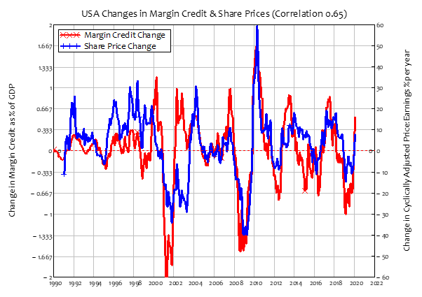
Secondly, as Janos Kornai emphasised (Kornai 1979; Kornai 1985), a firm in a competitive industry will have excess capacity in case one of its competitors stumbles, or in case its own marketing exceeds its expectations. Excess capacity is an essential element in the flexibility that a firm needs to be an effective competitor. Competition itself leads to this outcome, as individual firms collectively aim for shares of expected future sales that, in the aggregate, the entire industry cannot support: optimism about future sales and market share, rather than pessimism, is the default position for the managers of firms. This in itself leads to boom-bust cycles in most industries, which results in capacity utilization varying dramatically with the business cycle, while excess capacity is the rule at the aggregate level, as well as at the individual firm—see Figure 5.

Figure 5: Excess capacity in the USA never fell below 10%, even during the boom years of the late 60s https://fred.stlouisfed.org/series/TCU

As a factory expands output within its existing capacity, workers are hired in the proportion needed to bring idle machinery online. These machines are operated at the ideal ratio of variable inputs to fixed, rather than at above or below that ratio. Factories are also designed by engineers to be at their most efficient at full capacity, so as this level is approached, productivity per head will rise rather than fall.

A telling instance of this is recorded in Tesla’s 10K filing for January 2021, in which it noted that a lower level of output of solar roofs than planned led to higher unit costs and therefore much lower gross margins. Higher sales would have enabled a lower per-unit cost of production, and therefore a higher margin:

Gross margin for energy generation and storage decreased from 12% to 1% in the year ended December 31, 2020 as compared to the year ended December 31, 2019 primarily due to a higher proportion of Solar Roof in our overall energy business which operated at lower gross margins as a result of temporary manufacturing underutilization during product ramp.

In fact, the textbook story of a factory with more workers than are ideal for its installed capital is so far from reality that it is better described, not as a model, but as a (fractured) fairy tale.

In the real world, a well-designed and managed factory does not operate in the range where diminishing marginal productivity might apply—contrary to the assumptions of Neoclassical economists. Individual machines within that factory are also operated at their ideal variable input to fixed input ratio at all times (though the speed of operation may be varied as well—with higher speed bringing the machine closer to its optimum operating parameters, and if they are at the optimum, output is expanded by bringing more machines online). Consequently, as Sraffa put it in 1926:

Businessmen, who regard themselves as being subject to competitive conditions, would consider absurd the assertion that the limit to their production is to be found in the internal conditions of production in their firm, which do not permit of the production of a greater quantity without an increase in cost. (Sraffa 1926, p. 543)

Sraffa’s expectation was born out by a host of surveys, the last of which was undertaken by Alan Blinder. Mainstream economists have turned avoiding learning from these surveys into an art form. The most sublime such artwork is Blinder turning a blind eye his own research, but the most impactful was Friedman’s advice to economists to ignore similar research undertaken in the 1940s and 1950s.

Not Listening About Prices

A leading figure in this empirical research was Wilford Eiteman, who was both an academic economist and a businessman. This juxtaposition of roles led him to reject Neoclassical theory as factually incorrect:

Around 1940, Eiteman was teaching marginalism in principles of economics classes at Duke University when it occurred to him that as treasurer of a construction company he had set prices and talked with others who set prices and yet had never heard of any price-setter mentioning marginal costs. He quickly came to the conclusion that a price-setting based on equating marginal costs to marginal revenue was nonsense. (Lee 1998, Kindle Locations 1529-1531)

As well as writing papers on the logical reasons for declining marginal costs, Eiteman’s research (Eiteman 1945, 1947, 1948, 1953; Eiteman and Guthrie 1952) included a survey that presented the managers of firms with 8 drawings representing possible shapes of their short run average cost function. Only one of these matched the standard drawings in economics textbooks—see Figure 6.

Figure 6: Eiteman’s 3rd of 8 possible shapes for the average cost curve

Another two matched the situation that Eiteman knew from personal experience, of declining average costs right out to full capacity, or very near it—see Figure 7.

Figure 7: Eiteman’s 6^th and 7^th possible shapes for the average cost curve

Precisely one of Eiteman’s 334 survey respondents chose Figure 6. 203 nominated his 7^th drawing as properly representing their average costs, while another 113 opted for his 6^th. Amusingly, while Neoclassical economists see themselves as supporters of capitalism, actual capitalists, when informed of Neoclassical economic theory, thought Neoclassical economists were trying to undermine capitalism rather than support it. Eiteman noted this reaction by one businessman:

“‘The amazing thing is that any sane economist could consider No. 3, No. 4 and No. 5 curves as representing business thinking. It looks as if some economists, assuming as a premise that business is not progressive, are trying to prove the premise by suggesting curves like Nos. 3, 4, and 5.” (Eiteman and Guthrie 1952, p. 838)

Another critic, Richard Lester, asked his respondents at what level of output did they achieve maximum profits. All gave answers that contradicted the standard textbook model, with 80% of those answering reporting that maximum profits came at maximum output:

In the present study, a series of questions was asked regarding unit variable costs and profits at various rates of output. In reply to the question, “At what level of operations are your profits generally greatest under peacetime conditions?” 42 firms answered 100 per cent of plant capacity. The remaining 11 replies ranged from 75 to 95 per cent of capacity. (Lester 1946, p. 68)

These papers led to one of the most influential innovations in the history of economics. No, not a realistic model of the firm, obviously, but a methodological innovation: Milton Friedman’s mantra that “the more significant the theory, the more unrealistic the assumptions” (Friedman 1953, p. 153). Two of Friedman’s objectives with this paper were to stop research into models of the firm other than the two Neoclassical extremes of perfect competition and perfect monopoly, and to get economists to ignore empirical research challenging the assumption of diminishing marginal productivity:

The theory of monopolistic and imperfect competition is one example of the neglect in economic theory of these propositions. The development of this analysis was explicitly motivated .. by the belief that the assumptions of “perfect competition” or “perfect monopoly” said to underlie neoclassical economic theory are a false image of reality. And this belief was itself based almost entirely on the directly perceived descriptive inaccuracy of the assumptions rather than on any recognized contradiction of predictions derived from neoclassical economic theory. The lengthy discussion on marginal analysis in the American Economic Review some years ago is an even clearer, though much less important, example. The articles on both sides of the controversy largely neglect what seems to me clearly the main issue – the conformity to experience of the implications of the marginal analysis – and concentrate on the largely irrelevant question whether businessmen do or do not in fact reach their decisions by consulting schedules, or curves, or multivariable functions showing marginal cost and marginal revenue. (Friedman 1953, pp. 153-54. Emphasis added)

Friedman mischaracterised both of these research programmes, but especially the latter. He described the empirical research as being about whether businessmen actually use calculus in deciding output levels, when in fact it was about whether the conditions for this approach to work in the first place actually held. But this nuance didn’t matter to either Friedman, or the vast majority of Neoclassical economists, who simply did not want to hear what the empirical research was finding. They wanted to stick with their models of perfect competition and rising marginal cost, and Friedman’s methodological trick gave them a generic methodological reason to do so. When someone objected to the unreality of the model, they could sagely reply that it doesn’t matter that the assumptions of the theory of the firm are unrealistic, since “the more significant the theory, the more unrealistic the assumptions”:

the relation between the significance of a theory and the “realism” of its “assumptions” is almost the opposite of that suggested by the view under criticism. Truly important and significant hypotheses will be found to have “assumptions” that are wildly inaccurate descriptive representations of reality, and, in general, the more significant the theory, the more unrealistic the assumptions (in this sense)…

To put this point less paradoxically, the relevant question to ask about the “assumptions” of a theory is not whether they are descriptively “realistic,” for they never are, but whether they are sufficiently good approximations for the purpose in hand. And this question can be answered only by seeing whether the theory works, which means whether it yields sufficiently accurate predictions. The two supposedly independent tests thus reduce to one test. (Friedman 1953, p. 153. Emphasis added)

This is methodological nonsense. While it is passably true for genuine simplifying assumptions, it is utterly false when applied to justify assuming that firms experience rising marginal cost, when as a matter of empirical fact, they face constant or falling marginal cost.

A simplifying assumption is something which, if you don’t make it, results in a much more complicated model, which yields only a tiny improvement in its results over the simpler model.

For example, the Aristotelian belief that heavy objects fall faster than light ones was disproved by Galileo’s experiment, which showed that two dense objects of different weights fell at the same speed. Aristotelian physicists could have rejected Galileo’s proof on the grounds that his experiment ignored the effect of the air on how fast the objects fell. This would have forced Galileo to construct a much more elaborate experiment, but the outcome would have been almost exactly the same: the two objects of different weights would still have fallen at much the same rate, rather than the different rate that Aristotelian physics predicted. Galileo’s “assumption” that the experiment was conducted in a vacuum—which is easily classified as a “wildly inaccurate descriptive representation… of reality” (Friedman 1953, p. 153)—was a genuine simplifying assumption.

However, the assumption of rising marginal cost is instead an instance of what philosopher Alan Musgrave described as “domain assumptions” (Musgrave 1981). These are assumptions which, If they are true, mean that the theory applies, but if they are false, then it doesn’t. The assumption that marginal cost rises is not a mere simplifying assumption, but an assumption that is of critical importance to Neoclassical economic theory. If the assumption is false—which it manifestly is—then so is Neoclassical economics.

The critical importance of unrealistic assumptions

The Neoclassical profit maximization rule is to equate marginal revenue to marginal cost, assuming that the firm is producing past the point where average and marginal costs are rising. If marginal cost is rising, then marginal cost lies above average cost, and the firm makes a profit on every unit sold, right up until the point at which marginal cost equals price. For this reason, the marginal cost curve of a firm in a “perfectly competitive” industry is its supply curve: name a price, draw a line from that price out to the marginal cost curve, and the quantity the firm will supply at that price will be the quantity that equates its marginal cost to its marginal revenue, and thus maximizes its profit see (but see Keen and Standish 2010).

If marginal cost is falling however, then marginal cost is less than average cost. For the firm in a “perfectly competitive” industry, following the Neoclassical “profit-maximising” rule of equating marginal revenue to marginal cost results in a price that is therefore below average cost. At that price, the firm’s profit-maximising output level is zero. Therefore, there is no “supply curve” unless marginal cost is rising.

This is why Blinder’s empirical finding—that, for roughly 90% of firms, marginal cost is constant or falling right out to capacity output—was, as he put it, “overwhelmingly bad news … for economic theory”. This empirical fact means that the whole edifice of the Neoclassical theory of supply has to go. But that wasn’t what Blinder was looking for, let alone expecting, when he decided to ask firms about prices.

Asking About Prices—and then ignoring the answers

Hall and Hitch (Hall and Hitch 1939), Eiteman (Eiteman 1945, 1947, 1948; Eiteman and Guthrie 1952; Eiteman 1953), Lester (Lester 1946, 1947), Means (Means 1935, 1936, 1972; Tucker et al. 1938), and many others who have undertaken surveys of firms were critics of the Neoclassical model, and wanted to replace it with something more realistic. Blinder, au contraire, is solidly part of the Neoclassical establishment. His reason for undertaking his survey was not to question the mainstream, but to provide a firm foundation for “sticky prices”, which were an essential element of the “New Keynesian” faction of Neoclassical macroeconomists.

Self-described “New Classical” macroeconomists developed the approach of deriving macroeconomics directly from microeconomics, in which they assumed perfect competition throughout—and therefore, price equal to marginal cost. With rapid price adjustments, all of the impact of a change in aggregate demand was absorbed by a change in prices. In “Real Business Cycle” models therefore, the economy is in general equilibrium at all times, even during events like the Great Depression. Edward Prescott, one of the two originators of RBC modelling, argued that the cause of the huge rise in unemployment during the Great Depression was a voluntary decrease in the total number of hours of work that workers decided to supply, in response to unspecified changes in labour market regulations:

the Great Depression is a great decline in steady-state market hours. I think this great decline was the unintended consequence of labor market institutions and industrial policies designed to improve the performance of the economy. Exactly what changes in market institutions and industrial policies gave rise to the large decline in normal market hours is not clear. (Prescott 1999, p. 6)

This was too much for Neoclassical economists with some attachment to reality: unemployment during the Great Depression was not a utility-maximizing choice, but involuntary. Consequently, they developed Dynamic Stochastic General Equilibrium (DSGE) models, in which the slow adjustment of prices to equilibrium values was a key explanation of periods of involuntary unemployment. Blinder’s research was undertaken to find an empirically valid explanation for so-called “sticky prices”, within the overall confines of Neoclassical microeconomics:

In recent decades, macroeconomic theorists have devoted enormous amounts of time, thought, and energy to the search for better microtheoretic foundations for macroeconomic behavior. Nowhere has this search borne less fruit than in seeking answers to the following question: Why do nominal wages and prices react so slowly to business cycle developments? In short, why are wages and prices so “sticky”? The abject failure of the standard research methodology to make headway on this critical issue in the microfoundations of macroeconomics motivated the unorthodox approach of the present study. (Blinder 1998, p. 3)

The unorthodox aspect of his study was to actually conduct interviews—given that Friedman had disparaged the very idea of asking businessmen what they thought about their businesses:

The billiard player, if asked how he decides where to hit the ball, may say that he “just figures it out” but then also rubs a rabbit’s foot just to make sure; and the businessman may well say that he prices at average cost, with of course some minor deviations when the market makes it necessary. The one statement is about as helpful as the other, and neither is a relevant test of the associated hypothesis. (Friedman 1953, p. 158)

Blinder designed his study well to avoid the pitfalls expected by Friedman, so its results could not be dismissed as due to bad research procedures—and these results were similar to those reached by the earlier surveys that Friedman recommended economists not to read. But though Blinder knew his research methods were beyond reproach, he still found it hard to accept two of its key findings, that average fixed costs are high relative to average variable costs, and that marginal cost does not rise for the typical firm:

Third, firms typically report fixed costs that are quite high relative to variable costs (question AI2). And they rarely report the upward-sloping marginal cost curves that are ubiquitous in economic theory. Indeed, downward-sloping marginal cost curves are more common, according to the survey responses (question B 7 [a] ). If these answers are to be believed—and this is where we have the gravest doubts about the accuracy of the survey responses—then the whole presumption that prices should be strongly pro-cyclical is called into question. (Blinder 1998, p. 302)

His very next sentence showed why he had difficulty in accepting these answers. If they were true, then much of mainstream economic theory was false:

But so, by the way, is a good deal of microeconomic theory. For example, price cannot approximate marginal cost in a competitive market if fixed costs are very high. (Blinder 1998, p. 302)

In the end, fealty to conventional theory trumped Blinder’s personal exposure to the contrary data of facts. His denial of his own research findings in his textbook is so remarkable as to be worth citing at length:

The “law” of diminishing marginal returns, which has played a key role in economics for two centuries, states that an increase in the amount of any one input, holding the amounts of all others constant, ultimately leads to lower marginal returns to the expanding input.

This so-called law rests simply on observed facts; economists did not deduce the relationship analytically. Returns to a single input usually diminish because of the “law” of variable input proportions. When the quantity of one input increases while all others remain constant, the variable input whose quantity increases gradually becomes more and more abundant relative to the others, and gradually becomes over-abundant. (For example, the proportion of labor increases and the proportions of other inputs, such as lumber, decrease.) As Al uses more and more carpenters with fixed quantities of other inputs, the proportion of labor time to other inputs becomes unbalanced. Adding yet more carpenter time then does little good and eventually begins to harm production. At this last point, the marginal physical product of carpenters becomes negative.

Many real-world cases seem to follow the law of variable input proportions. In China, for instance, farmers have been using increasingly more fertilizer as they try to produce larger grain harvests to feed the country’s burgeoning population. Although its consumption of fertilizer is four times higher than it was fifteen years ago, China’s grain output has increased by only 50 percent. This relationship certainly suggests that fertilizer use has reached the zone of diminishing returns. (Baumol and Blinder 2015, p. 124. Emphasis added)

Blinder’s claim that the “law” was implied from empirical observation, rather than derived deductively, is simply untrue. The concept was first put in its Neoclassical form in 1911 by Edgeworth, where his table was, like Mankiw’s alliterated firms in today’s textbooks, a figment of Edgeworth’s imagination. To illustrate how mistaken Blinder is above, it is also worth quoting at length from Brue’s careful examination of the intellectual history of the concept of diminishing returns:

an explicit exposition of diminishing returns, distinguishing between the average and marginal products of a variable homogeneous input, had to await Francis Edgeworth and John Bates Clark.

In 1911 Edgeworth constructed a hypothetical table in which he assumed land was a fixed input (Edgeworth 1911, p. 355). The first two columns of the table related various levels of the “labor/tools” input with corresponding levels of total crops. In the third column, Edgeworth derived the marginal product of the variable input; in the fourth, the average product of the variable input. Thus, the values of the table demonstrated the relationships between total, marginal, and average product. Like his predecessors, Edgeworth drew his example from agriculture, not manufacturing. Nevertheless, he asserted that the idea was applicable in all industries…

Jacob Viner (1931 [1958], pp. 50–78) and others then developed the contemporary graphical link between the law of diminishing marginal returns and the firm’s marginal cost curves and short-run product supply curves. Since then, the law of diminishing returns has become the modern centerpiece for explaining upward-sloping product supply curves…

Along with circular and special-case proofs, none of the economists mentioned here marshalled strong empirical evidence to validate their propositions. Instead they stated the law as an axiom, offered specific examples, or referred to hypothetical data to demonstrate their point…

Menger (1936 [1954]) severely criticized the axiomatic acceptance of the law of diminishing returns, arguing that the crucial issue for economics is the empirical question of whether or not the laws of returns are true or false. His call for direct empirical verification of the law—and through extension, the rising short-run marginal cost curve—remains valid.

In his 1949 book Manufacturing Business, Andrews (pp. 82–111) introduced another complication relating to the law of diminishing returns and its applications. He argued that manufacturing firms maintain excess capacity so that they do not lose present customers in times of unexpected demand, have the capacity to cover for breakdowns of machinery, and take advantage of opportunities to capture new customers in a growing market. When excess capacity exists, the law of diminishing returns may have little relevance for cost curves. Firms can change short-run output simply by varying the hours of employment of the “fixed” plant proportionally with the variable inputs. The ratios of the inputs employed need not change and marginal cost need not rise…

However, it does seem clear that the history of economic theory has produced an axiomatic acceptance of the law of diminishing returns and rising marginal costs. More empirical investigation is needed on whether this law is operational under conditions of excess capacity, and how it is relevant to the burgeoning service industries. Conjectures by 19th century economists about input and outputs in agriculture simply won’t do! (Brue 1993, pp. 187-91. Emphasis added)

Blinder’s own examples also contradict his statement that “diminishing marginal returns” rests on “observed facts”. His first example is a fictional one, from his made-up example of Al’s Building Company. His second example, of the increased use of fertilizer in China over 15 years, violates the pre-conditions of diminishing marginal productivity, which only apply in the short-run when one factor of production is fixed.

This argument reeks of Blinder attempting to rationalise ignoring the results of his own research. His unexpected experience of what Thomas Huxley elegantly described as “the great tragedy of Science—the slaying of a beautiful hypothesis by an ugly fact” (Huxley 1870, p. 402), led to him to discard the ugly fact, so that he could remain faithful to the beautiful theory.

In fact, the theory is anything but beautiful, as a more critical examination of Blinder’s and Mankiw’s fictional examples exposes—see the Appendix. But the main problem is that it is simply wrong. Our theory of costs and prices should be based on reality rather than fantasy.

Real Cost Curves

The consistent points found in empirical research about actual firms are that:

• Average Fixed Costs are high. Whereas Neoclassical drawings—for that is all they are— put average fixed cost at 10-20% of total costs at maximum output, only ¼ of the firms Blinder surveyed picked a figure below 20%. The mean value was 44% of total costs, and 8% of firms reported average fixed costs at over 80% of total costs;
• Average Variable Costs are commensurately lower than in Neoclassical drawings, and generally fall rather than rise as output rises.
• Therefore, Marginal Cost typically lies below Average Variable Cost, and well below Average Total Cost.

Figure 8 shows an extreme example of this empirical norm—using hypothetical data, because I don’t have access to commercial data, but with the characteristics of this hypothetical case fitting Blinder’s survey results, rather than contradicting them, as Blinder does in his textbook. These are cost curves for a silicon wafer manufacturing firm, based loosely on Samsung’s major plant, with Fixed Costs of $33 billion, an assumed cost of capital of 5% (the same as Mankiw used in his examples), Average Fixed Costs being 85% of total costs at maximum output, and declining variable costs, beginning at $1600 per wafer and falling to $1344 at capacity output of 744,000 wafers per year. This is roughly consistent with price being an estimated 100% markup on costs per wafer, and prices in the realm of $5000 per wafer for high-end wafers.

Figure 8: Hypothetical costs for a silicon wafer foundry

Marginal cost is irrelevant to the output decision here, while the profit-maximizing output level is 100% of capacity. Price also far exceeds marginal cost.

Neoclassical economics could cope with this situation if it could regard this as an example of a “natural monopoly”, where declining costs make a competitive structure impossible—but the numerous surveys have all found that the vast majority of firms in all industries report a similar cost structure. This implies that price both substantially exceeds marginal cost, and is indeed unrelated to it, in all industry structures.

What the theory of supply should be

The false Neoclassical assumption of diminishing marginal productivity is a critical component of the Neoclassical theory of supply. It goes hand in hand with the eulogising of “perfect competition”, the demonising of “monopoly”, and the analysis of intermediate structures—”imperfect competition”, “oligopoly”—by means of game theory. It is vital to the claim that competitive markets achieve a social optimum of marginal benefit equalling marginal cost, and that other market structures are inferior because they result in output levels where marginal benefit exceeds marginal cost.

It is also a serious impediment to understanding real competition. In the real world, where almost all firms face declining average costs as output rises, and market capacity significantly exceeds market demand in normal times, the emphasis is on achieving higher sales than the breakeven level, and targeting the maximum sales volume possible. This is done via product development and differentiation, aided by marketing that focuses on the qualitative differences between the firm’s product and those of its competitors. Falling average cost with production volume gives the firm capacity to discount as sales increase, and allow price to fall as sales rise—the opposite of the Neoclassical model, and consistent with the results of numerous surveys of business practice.

This real process of competition could explain why the real world size distribution of firms bears absolutely no resemblance to the Neoclassical taxonomy of “perfectly competitive, imperfectly competitive, oligopolistic, monopolistic” industries, but instead has many small firms co-existing in industries with a few large firms. This empirical regularity (which is known as a Power Law, Zipf Law or Pareto Law distribution), results in the log of a measure of the size of a firm being negatively related to the log of how many firms are that size in an industry or country (Axtell 2001, 2006; Fujiwara et al. 2004; Heinrich and Dai 2016; Montebruno et al. 2019).

This is readily seen in the aggregate US data—see Table 3, which shows the 2014 data from the United States Small Business Administration (SBA) on the number of firms by the number of employees per firm (the data covers all firms in the USA, but the SBA provides detailed statistics only for firms with 500 or less employees).

Table 3: Number of US firms and size of firms in 2014 (https://www.sba.gov/sites/default/files/advocacy/static_us_14.xls)

Figure 9 shows the characteristic linear relationship between the log of size and log of frequency that turns up in Power Law distributions.

Figure 9: The Power Law behind the size distribution data in Table 3

This kind of distribution abounds in nature as well as in economic data (Axtell 2001; Di Guilmi et al. 2003; Malamud and Turcotte 2006; Gabaix 2009). It is the hallmark of the evolutionary dynamics that should be the focus of economics, in marked contrast to the sterile taxonomy of non-existent industry market structures that both defines and bedevils Neoclassical microeconomics.

Conclusion

The Neoclassical theory of the supply curve as the sum of the rising marginal cost curves of firms in a perfectly competitive industry is thus a fiction, right from the foundational concept of diminishing marginal productivity. Its origins lie, not in the real world, but in its role as a reflection of the Neoclassical theory of the demand curve, where “diminishing marginal utility” is the foundational concept. When diminishing marginal utility in a rational, utility maximizing consumer, meets diminishing productivity in a rational, profit-maximizing firm, we get the Neoclassical nirvana of marginal benefit equalling marginal cost, and therefore free-market capitalism as the social system that best maximises utility, subject to the cost constraint.

This is why Neoclassicals cling so religiously to the concepts of diminishing marginal productivity, and rising marginal cost, despite overwhelming empirical evidence to the contrary (Sraffa 1926; Hall and Hitch 1939; Eiteman 1947; Eiteman and Guthrie 1952; Means 1972; Blinder 1998; Lee 1998). If they admit that the norm is constant or rising marginal productivity, and constant or falling marginal cost, then the two halves of Neoclassical economics no longer fit together. Better bury the empirical evidence (Friedman 1953) or ignore it (Baumol and Blinder 2015), rather than to accept it, and have to abandon Neoclassical economics instead.

We should have no such qualms. The Neoclassical theory of the firm is the economic equivalent of the theory of Phlogiston that chemists once used to explain combustion, before the discovery of oxygen. Economists discovered their oxygen almost a century ago now, firstly in the logical work of Sraffa in 1926 (Sraffa 1926) and then the empirical work of the Oxford Economists’ Research Group, which commenced in 1934 (Lee 1998, Chapter 4). It’s well past time that we threw out the economic equivalent of Phlogiston, the belief in “diminishing marginal productivity” as a characteristic of industrial capitalism, and developed a realistic theory of firms, industries, and competition.

And if this involves abandoning Neoclassical economics as well, then so much the better.

Appendix: The real shape of fictional cost curves

You will recall that shows Table 2 shows the per-unit costs that can be derived from Mankiw’s fictional production data for “Caroline’s Cookie Factory”, shown in Table 1. Figure 10 graphs those numbers. This Figure has characteristics that should be readily apparent to anyone who has ever even glanced at an economics textbook.

Figure 10: Cost curves derived from Mankiw’s production numbers in Table 1

Firstly, this diagram is ugly: it looks nothing like the (relatively) beautiful curves Mankiw shows for cost curves in the same chapter—see Figure 1, Error! Reference source not found. and Error! Reference source not found. here. They all look fine in comparison to Figure 10.

Secondly, notice that the numbers on Figure 1 are very small—maxing out at 10 units per hour—while there are no numbers on the axes of Error! Reference source not found. or Error! Reference source not found.. Why not?

The clue to this puzzle is the values on the Quantity axis for Mankiw’s total cost curve plot (Figure 11 below), and the Quantity axis for his demonstration of rising marginal cost (Figure 12). Notice that the Quantity Axis for “Hungry Helen’s” total cost curve Figure 11 has a maximum of 150 units per hour—not a big number, but OK if we’re imagining a numerical example of a single firm in a “perfectly competitive” market.

Figure 11: Mankiw’s Figure 13-3, on page 275

Now check the Quantity axis on Figure 12, which supposedly shows the cost structure for another “typical” firm, “Thirsty Thelma’s”: it maxes out at just ten units per hour: a decidedly small number. Why doesn’t Mankiw use a more reasonable number, like he did in the penultimate figure?

Figure 12: Mankiw’s Figure 13-5, on page 279

It gets curiouser still. Mankiw has not one graph of total cost, but two—see Figure 11 and Figure 13. Why?

Figure 13: Mankiw’s Figure 13-4, on page 276

It is, I expect, because Mankiw tried using the data from “Hungry Helen’s” to derive the average and marginal cost curves, but found that the graph looked ugly—it looked, in other words, like my Figure 10. This simply wouldn’t do in a textbook that pays more attention to appearance than its content, so he tried lower numbers for another made-up firm, “Thirsty Thelma’s”, and that worked. Rather than getting rid of the whole previous section—with “Hungry Helen’s” higher output numbers—he just left it in there, resulting in two superficially identical figures for Total Cost. Again, why?

This puzzle has a numerical solution, which explains a bizarre feature of Neoclassical textbook examples of the cost structure of firms: when they show drawings derived from made-up data, the quantity numbers are trivial. Mankiw, as noted, has a maximum output of ten units per hour in his “Thirsty Thelma’s” example (see Figure 12); Blinder has 10 garages per year as his maximum output level for the cost curves in “Al’s Building Company” (Baumol and Blinder 2011, pp. 132-134)—see Figure 4—even though he earlier had his fictional company producing up to 35 garages per year in his exposition of the production function (Baumol and Blinder 2011, p. 124).

The answer is that the shapes of archetypical average and marginal cost drawings that abound in Neoclassical texts—where Average Variable Costs are about five times Average Fixed Costs at the maximum output level shown on the drawing, while the rapidly-falling segment of Average Fixed Cost is also visible on the diagram—require Fixed Cost to be very small. If large output numbers are used, the resulting curves will look nothing like the archetypical shape.

To understand this, firstly note that, since marginal cost and variable cost curves are treated as continuous functions, they can be approximated by polynomials. Secondly, marginal cost (MC) is the derivative of variable cost (VC) with respect to quantity Q, and average cost (AVC) is variable cost VC divided by Q: see Equations and :

         

         

Since AVC and MC can be expressed as polynomials, they are therefore polynomials of the same order: all they differ by are their coefficients. In turn, these coefficients are related by a simple rule, that the coefficient for the n^th power of a marginal cost term must be times the coefficient for the same term in average variable cost. For example, if marginal cost (MC) is a quadratic, then so is average variable cost (AVC), and the coefficient for the term in MC will be three times the coefficient for the term in AVC—see Equation :

         

Average Fixed Cost AFC, on the other hand, is a reciprocal function:

         

To make polynomial functions of Q appear on the same scale as an inverse function of Q, the value of Q can’t be too big—hence the crazily small numbers used for output in numerically derived Neoclassical drawings. I doubt that this numerical fudging was deliberate, because Neoclassicals are not aware of these limitations on the shape of cost functions for their preferred model. I suspect instead that these authors tried arbitrarily chosen values for Fixed Cost with large values for , unexpectedly got ugly drawings like Figure 10, and went on to use smaller values for , without realising why those drawings worked better than those with larger values.

References

Axtell RL (2001) Zipf Distribution of U.S. Firm Sizes. Science (American Association for the Advancement of Science) 293 (5536):1818-1820. doi:10.1126/science.1062081

Axtell RL (2006) Firm Sizes: Facts, Formulae, Fables and Fantasies.

Baumol WJ, Blinder A (2011) Microeconomics: Principles and Policy. 12th edn.,

Baumol WJ, Blinder AS (2015) Microeconomics: Principles and policy. 14th edn. Nelson Education,

Blinder AS (1998) Asking about prices: a new approach to understanding price stickiness. Russell Sage Foundation, New York

Brue SL (1993) Retrospectives: The Law of Diminishing Returns. Journal of Economic Perspectives 7 (3):185-192. doi:10.1257/jep.7.3.185

Di Guilmi C, Gaffeo E, Gallegati M (2003) Power Law Scaling in the World Income Distribution. Economics Bulletin 15 (6):1-7. doi:http://www.economicsbulletin.com/

Edgeworth FY (1911) Contributions to the Theory of Railway Rates. The Economic journal (London) 21 (83):346-370. doi:10.2307/2222325

Eiteman WJ (1945) The Equilibrium of the Firm in Multi-Process Industries. THE QUARTERLY JOURNAL OF ECONOMICS 59 (2):280-286

Eiteman WJ (1947) Factors Determining the Location of the Least Cost Point. The American Economic Review 37 (5):910-918

Eiteman WJ (1948) The Least Cost Point, Capacity, and Marginal Analysis: A Rejoinder. The American Economic Review 38 (5):899-904

Eiteman WJ (1953) The Shape of the Average Cost Curve: Rejoinder. The American Economic Review 43 (4):628-630

Eiteman WJ, Guthrie GE (1952) The Shape of the Average Cost Curve. The American Economic Review 42 (5):832-838

Friedman M (1953) The Methodology of Positive Economics. In: Essays in positive economics. University of Chicago Press, Chicago, pp 3-43

Fujiwara Y, Di Guilmi C, Aoyama H, Gallegati M, Souma W (2004) Do Pareto–Zipf and Gibrat laws hold true? An analysis with European firms. Physica A 335 (1):197-216. doi:10.1016/j.physa.2003.12.015

Gabaix X (2009) Power Laws in Economics and Finance. Annual Review of Economics 1 (1):255-293. doi:http://arjournals.annualreviews.org/loi/economics/

Garrett TJ, Grasselli M, Keen S (2020) Past world economic production constrains current energy demands: Persistent scaling with implications for economic growth and climate change mitigation. PLoS ONE 15 (8):e0237672. doi:https://doi.org/10.1371/journal.pone.0237672

Hall RL, Hitch CJ (1939) Price Theory and Business Behaviour. Oxford Economic Papers (2):12-45

Heinrich T, Dai S (2016) Diversity of firm sizes, complexity, and industry structure in the Chinese economy. Structural change and economic dynamics 37:90-106. doi:10.1016/j.strueco.2016.01.001

Huxley TH (1870) Address of Thomas Henry Huxley, L.L.D., F.R.S., President. Nature 2 (46):400-406

Keen S (2004) Deregulator: Judgment Day for Microeconomics. Utilities Policy 12:109-125

Keen S (2005) Why Economics Must Abandon Its Theory of the Firm. In: Salzano M, Kirman A (eds) Economics: Complex Windows. New Economic Windows series. Springer, Milan and New York: , pp 65-88

Keen S, Ayres RU, Standish R (2019) A Note on the Role of Energy in Production. Ecological Economics 157:40-46. doi:https://doi.org/10.1016/j.ecolecon.2018.11.002

Keen S, Standish R (2006) Profit maximization, industry structure, and competition: A critique of neoclassical theory. Physica A: Statistical Mechanics and its Applications 370 (1):81-85

Keen S, Standish R (2010) Debunking the theory of the firm—a chronology. Real World Economics Review 54 (54):56-94

Kornai J (1979) Resource-Constrained versus Demand-Constrained Systems. Econometrica 47 (4):801-819

Kornai J (1985) Fix-Price Models: A Survey of Recent Empirical Work: Comment. In: Arrow KJ, Honkapohja S (eds) Frontiers of Economics. Oxford and New York:

Blackwell, pp 379-390

Lee FS (1998) Post Keynesian Price Theory. Cambridge University Press, Cambridge

Lester RA (1946) Shortcomings of Marginal Analysis for Wage-Employment Problems. The American economic review 36 (1):63-82

Lester RA (1947) Marginalism, Minimum Wages, and Labor Markets. The American economic review 37 (1):135-148

Malamud BD, Turcotte DL (2006) The applicability of power-law frequency statistics to floods. Journal of Hydrology 322 (1-4):168-180. doi:DOI: 10.1016/j.jhydrol.2005.02.032

Mankiw NG (2001) Principles of Microeconomics. 2nd edn. South-Western College Publishers, Stamford

Mankiw NG (2009) Principles of Microeconomics. 5th edn. South-Western College Publishers, Mason, OH

Means GC (1935) Price Inflexibility and the Requirements of a Stabilizing Monetary Policy. Journal of the American Statistical Association 30 (190):401-413

Means GC (1936) Notes on Inflexible Prices. The American Economic Review 26 (1):23-35

Means GC (1972) The Administered-Price Thesis Reconfirmed. The American Economic Review 62 (3):292-306

Montebruno P, Bennett R, Van Lieshout C, Smith H (2019) A tale of two tails: Do Power Law and Lognormal models fit firm-size distributions in the mid-Victorian era? doi:10.17863/CAM.37178

Musgrave A (1981) ‘Unreal Assumptions’ in Economic Theory: The F‐Twist Untwisted. Kyklos (Basel) 34 (3):377-387. doi:10.1111/j.1467-6435.1981.tb01195.x

Prescott EC (1999) Some Observations on the Great Depression. Federal Reserve Bank of Minneapolis Quarterly Review 23 (1):25-31

Sraffa P (1926) The Laws of Returns under Competitive Conditions. The Economic Journal 36 (144):535-550

Tucker RS, Bernheim AL, Schneider MG, Means GC (1938) Big Business, Its Growth and Its Place. Journal of the American Statistical Association 33 (202):406-411

 

 

If you’ve read my previous posts on Ravel (one, two, three), you’ll know that I’m making the current beta available to Patrons on my 68^th birthday, which is tomorrow: March 28^th. This post covers:

• What I’d like Patrons to do with Ravel, which includes:
  • Share it with friends—I actually want to get Ravel into as many people’s hands as possible—while respecting both their privacy and mine;
  • Test using Ravel for data analysis that you customarily do using other programs, whether that’s just Excel, or something as advanced and complicated as R; and
  • Give me and Russell Standish, who’s programmed Ravel into existence, feedback on it;
• How Ravel came about; and
• Why we’re sharing it now, rather than waiting until a commercial version is ready.

Share it

I’ll start with the second topic first. Though I’m making this beta available to Patrons only, I’d actually like to get it into as many hands as possible. So I actually want my patrons to share it with friends—but preferably, in a way that lets us gather the names and addresses of potential purchasers of a commercial version of Ravel, much further down the track.

We were going to do this automatically via an online web store, but Russell has checked out about six open-source stores, and they have all sucked, in one way or another. So tomorrow, we are going to simply give you an URL from which you or anyone else can download the current beta of Ravel.

To share it with friends, all you have to do is send them the URL—but please, ask first if they’re willing to share their names and email addresses with us. If they’re not, but you still want to show it to them, and they are still curious, then share it anyway. Getting the product into circulation is more important to me than collecting addresses for the future marketing of the commercial release of Ravel.

We will continue releasing subsequent betas to Patrons, and I’d ask that you don’t share these with friends: instead, if anyone wants to use the latest version, tell them to sign up to Patreon, either here or at Minsky’s page at http://patreon.com/hpcoder/.

Test it

For obvious reasons, I use Ravel to analyze and display economic data. But it is a generic data analysis and display tool, which can handle anything that you can put into a CSV file (other file import formats will be supported over time). I’d especially like to hear people’s experiences in using it with corporate, government, or scientific data, since if it does reach the commercial stage, they will be a far larger part of the market than just academics.

There will be many limitations to Ravel compared to the programs you’re currently using, simply because we haven’t finished designing it yet. But we believe that the Ravel itself—a graphical way of displaying multi-dimensional data—is a significant advance over existing programs, and that coupling this with Minsky’s existing ability to design equations visually makes it a potential “killer app”. It can do what Pivot Tables do in Excel, and in fact can take over many of the functions of Excel itself. It is also easy to audit a Ravel sheet because the equations are graphical, and one equation can take the place of tens of thousands of cell references in Excel.

Figure 1: Using BIS Debt database to derive GDP and credit

Give us Feedback

Russell and I have been developing Ravel in our spare time for several years now. Most of our time has been taken up in getting the basic engine to work properly—design at one end, bug fixing at the other. Now that the basic features are in place, we need feedback from users about how it feels to use Ravel rather than other programs—primarily, Excel, plus Pivot Tables in Excel and other programs.

So please, use it and let us know what the experience is like. Replies to tomorrow’s post where we launch the program will be a good start; sometime soon we’ll organize a place to discuss it properly—perhaps a channel on Discord.

How Ravel Came About

Before I became an academic, I was a software reviewer for Australia’s two leading computing magazines—firstly Australian Computing, then Your Computer. Both are defunct now, but that role gave me exposure to the entire spectrum of computer software during what could be called its “Cambrian” phase: when there was an enormous amount of experimenting, and no overall dominant software provider.

Those halcyon days are long gone. Now Microsoft and Google between them dominate the program world. And, frankly, we’re much worse off for it, because many of the programs that have died in the meantime were far better than the programs that are dominant today. They didn’t necessarily look better—the cosmetic features of software have improved as operating systems and faster chips have allowed more processor cycles to go to appearance rather than substance—but they were functionally superior.

One of these programs was PC Express. Think a spreadsheet, but with up to a dozen axes rather than just two, with formulas that operated on entire arrays of data rather than individual spreadsheet cells. I loved this product, and raved about it. The one thing I criticized it for was the lack of an intuitive Graphical User Interface.

Figure 2: My review of PC Express, later reproduced by IRAUS as a promotional leaflet

Some years later, the Australian division of Information Resources International, IRAUS, asked me to give the keynote speech at their annual conference, and suggested that I focus on its weakness—the absence of a GUI. Could I think of one for the speech?

Inspired by Javelin, another program that I’d recently reviewed that had a much better GUI but nothing like PC Express’s power, I came up with what today we call a Ravel.

Figure 3: Part of my presentation for IRAUS’s AGM in 1989

I was in discussions with IRAUS and its international parent IRI to sell my interface idea to them and incorporate it into PC Express, when the program was purchased by Oracle, and everyone I was dealing with disappeared from the company.

The idea went into deep freeze as I continued on my academic career—which had started in 1987. Then in late 1995, I and several other Sydney-based specialists in complex systems decided to run a conference on the complex systems approach to economics, called Commerce, Complexity and Evolution.

Figure 4: The book produced from the conference Commerce, Complexity and Evolution

One of the people who submitted a paper to that conference was Dr Russell Standish, who was then Head of the High Performance Computing (HPC) Unit, a joint venture by the Universities of New South Wales and Sydney. Russell and I became close friends afterwards. A few years later, the Universities shut the HPC joint venture down, making Russell redundant. He decided to go into commercial programming rather than look for another university role, while I rose from a tutor at UNSW in 1987 to a Professor at the University of Western Sydney in the mid-2000s.

In the early 2010s, I developed the idea of building Minsky as a systems dynamics program, and got funding for it from the Institute for New Economic Thinking. My first choice for someone to program it was Russell, and luckily, he was available.

Then in late 2012, I copped the same fate as Russell had a decade earlier, when the University of Western Sydney decided to shut its economics department down and make me and the 4 other Professors of Economics redundant. Since Russell and I were already working together on Minsky, I suggested that we start developing Ravel as well. Unlike Minsky, Ravel was developed as a sideline and without any funding—apart from some of my retirement savings. So it’s been a very slow burn, and we took some wrong turns along the way (including designing it as an Excel plug-in). We finally settled on building it on top of Minsky’s GUI, and finally Ravel is at a point where we’re willing to put it into other people’s hands.

Why now?

Our original plan was to develop Ravel as a commercial venture, and use the revenue from it both for our own lifestyles, and also to fund the research that Russell and I have always wanted to do, but have never been able to raise the required funding. I also wanted to hang onto the development reins of Ravel, since over the years I’d seen so many good programs die because of bad management. I was damned if I was going to let that happen to Ravel.

Then I read the work of William Nordhaus and friends, and I realized that I didn’t have time to run a company, as well as take on their civilization-threatening trivialization of the dangers of climate change. Nonetheless, development of Ravel was still continuing, and by the time I’d published my first critique of Nordhaus, Ravel was almost ready for prime time.

Figure 5: My critique of Nordhaus, published in September 2020

There was one problem: its handling of large data sets. That was addressed by adding the capability to handle sparse data arrays, and the work to get that right was only finished a month or so ago.

If we were going to go the product sales route, we would have kept it in house until it was ready for a first commercial release. But now that we both realize the effort that has to be put into first raising the alarm about how much worse climate change will be than economists have claimed, and then developing alternative analysis, we are open to other avenues. In particular, there’s no point in delaying a release: so why not give it away on my birthday to my supporters on Patreon? It’s as good a reason as any to get Ravel into the hands of more users.

As Graeber pointed out in Debt: The First 5000 Years, the assumption that money originated in barter is an enduring myth in economics: “First comes barter, then money; credit only develops later” (Graeber 2011, Chapter 2). This myth permeates the discipline, from Adam Smith’s assertion in 1776 that “the propensity to truck, barter, and exchange one thing for another” (Smith 1776, Chapter 2) was an innate characteristic of humans, to modern economics textbooks, like Gregory Mankiw’s Macroeconomics, that argue that an economy without money would be “a barter economy” (Mankiw 2016, p. 82).

Armed with this myth, economists have constructed a fantasy model of capitalism in which money plays no significant role: it is a mere trifle that sensible economists look through, to see the real face of barter lying behind the veil of money. Consequently, mainstream economists ignore banks, debt and money, while credit plays no role in their mathematical models of the macroeconomy.

This is why they not only didn’t see the 2007 Global Financial Crisis coming, but in fact expected 2008 to be a cracker of a year. The OECD’s Economic Outlook in June 2007 trumpeted that “sustained growth in OECD economies would be underpinned by strong job creation and falling unemployment” (Cotis 2007, p. 5).

Yeah, right. Two months after this forecast was published, the biggest economic crisis before Covid-19 and since the Great Depression began.

Why were they so wrong? Because they ignore Graeber’s central message that debt and credit drive the development, and sometimes the collapse, of economies.

Their logic rests, as usual, on a naïve assumption. They assume that banks are simply “intermediaries” between people who save money, and people who borrow money, and therefore that redistributing this money has little effect on economic activity. As ex-Federal Reserve Chairman Ben Bernanke put it, “Absent implausibly large differences in marginal spending propensities among the groups … pure redistributions should have no significant macroeconomic effects.” (Bernanke 2000, p. 24).

What the hell does that jargon mean? It means that mainstream economists pretend that banks don’t create money when they lend—something that they can no longer do after The Bank of England categorically said that they do (McLeay, Radia et al. 2014)—or that this doesn’t really matter. A little arithmetic is enough to show they’re wrong, and David was right.

One of the incontrovertible truisms of economics is that your spending is someone else’s income: what is expenditure to you is income to someone else. For simplicity, imagine a three-person economy—Tom, Dick, and Harriet—where Tom spends $60 a year on Dick & $40 a year Harriet, Dick spends $30 a year on Tom and $90 a year on Harriet, and Harriet spends $70 a year on Tom and $60 a year on Dick. Total income and total expenditure in this toy economy, shown in Table 1, is therefore $350 per year.

Table 1

The mainstream economic fantasy that banks are “financial intermediaries”, can be illustrated by imagining that Dick lends $10 to Tom at 10% interest, and Tom uses this to spend another $10 on Harriet, while also having to pay Dick $1 interest. Do the sums on Table 2, and you’ll find that total income and total expenditure is $351: the $1 in interest has turned up as extra expenditure by Tom and income to Dick. But the $10 that Tom borrowed from Dick cancels out: to lend $10 to Tom for him to spend, Dick had to spend $10 less on Harriet.

Table 2

But what if Tom got a loan, not from Dick, but from the bank? This toy economy is closer to the real world. Here, the increase in Tom’s spending power comes from increasing his indebtedness to the bank. The additional $10 spending on Harriet does not come at the expense of Dick’s spending, as in the mainstream economics fantasy, but from the bank loan creating $10 of new money, which Dick then spends on Harriet. Include the bank also spending its $1 in interest income on Dick, and you will find that income and expenditure in this more realistic toy m    odel is $361: the credit money that the bank loan created has increased both expenditure (Tom’s, by $10) and incomes (Harriet’s, by $10).

Table 3

This simple monetarist arithmetic is what mainstream economists are ignoring when they leave banks, debt, and money out of their models. It’s why they have never seen an economic crisis coming, because they ignore what causes it: too much credit during a boom, and credit turning negative during a slump. Because of their fallacious advice to ignore the level of private debt and its growth (credit), policymakers ignored clear signs that a crisis was imminent in 2007. Then credit turned negative for the first time since WWII, and the OECD’s assurance that the world would experience “sustained growth” in 2008 was in tatters.

Figure 1: USA Private Debt and Credit since 1950

One of the great tragedies of 2020 is that David is no longer with us, but mainstream economics still is. We should honor his memory by, as he wished, killing the delusional fantasy that is mainstream economic theory. We should also bring to life the idea he, Michael Hudson and I have championed, of a Modern Debt Jubilee, to free us from our bondage to those who have profited out of this explosion of private debt: free us from those whom Marx aptly called “the Roving Cavaliers of Credit” (Marx 1894, Vol.3, Chapter 33).

Bernanke, B. S. (2000). Essays on the Great Depression. Princeton, Princeton University Press.

Cotis, J.-P. (2007). Editorial: Achieving Further Rebalancing. OECD Economic Outlook. OECD. Paris, OECD. 2007/1: 7-10.

Graeber, D. (2011). Debt: The First 5,000 Years. New York, Melville House.

Mankiw, N. G. (2016). Macroeconomics. New York, Macmillan.

Marx, K. (1894). Capital Volume III. Moscow, International Publishers.

McLeay, M., A. Radia and R. Thomas (2014). “Money creation in the modern economy.” Bank of England Quarterly Bulletin
2014 Q1: 14-27.

Smith, A. (1776). An Inquiry Into the Nature and Causes of the Wealth of Nations. Indianapolis, Liberty Fund.

 

Hands up if you’ve tried to use Pivot Tables in Excel, and given up?

Me too! Which is why Russell Standish and I have developed “Ravel“: a visual way to manipulate “multi-dimensional data”. On my birthday this year—March 28^th—we’re giving Ravel to our supporters on Patreon, as a “Hobbit” birthday present.

If you don’t know the reference, in Tolkien’s classics The Hobbit and The Lord of the Rings, the Hobbit having a birthday gave presents to all the other Hobbits at his or her birthday party. To be a Hobbit guest at my 68^th birthday party, please sign up to either https://www.patreon.com/ProfSteveKeen or http://patreon.com/hpcoder/.

This post is a quick explanation of what Ravel does, and how to use it.

Figure 1 shows a Ravel. This one has four Axes, or dimensions—Country, Sector, Unit, and Quarter. A Ravel can have as few as one Axis, and as many as you like.

Figure 1: A Ravel of the BIS database, with its data input parameter attached to its input port

This particular Ravel contains the Bank of International Settlements (BIS) database on debt. It has data on 43 countries, over 300 quarters (from the early 1940s until September 2020), with three sectors (Government, Households and Non-Financial Corporations), and three ways of showing the data (in domestic currencies, percent of GDP, and US dollars).

Figure 2 shows Ravel‘s user interface.

Figure 2: Ravel’s user interface

It’s Minsky‘s user interface, augmented by the Ravel itself (the second-last icon on the toolbar). You display and analyze the data in a Ravel by attaching its output port—the circle on the right-hand side of the Ravel, visible in Figure 1—to sheets, plots, and mathematical operators on the canvas.

It takes some work to get data like the BIS’s file into a Ravel (as I will explain in another post this week) but once you’ve done it, manipulating a Ravel is a breeze—far easier than manipulating a spreadsheet, let alone a Pivot Table.

For example, let’s say that you wanted to graph the USA’s household and corporate debt levels, as a percentage of the USA’s GDP, over time. Doing that with Excel involves selecting the USA’s data from the BIS’s CSV file (attached to this post), which starts in column AT on row 1072 (see Figure 3), aligning it with the quarterly date data on row 1, and … the remainder is left as an exercise for the reader (try defining a data table , sorting it by sector and filtering by country, selecting the USA, and …; you’ll get there, eventually).

Figure 3: USA sectoral debt to GDP ratios in Excel

Doing the same thing in Ravel involves moving the selector dot on the Country Axis to “USA”, and on the Unit Axis to “Percentage of GDP”, and then attaching a plot:

Figure 4: Selecting the USA and Percent of GDP on the Ravel in Figure 1 and attaching a plot

What if you want to look at total private sector debt to GDP ratios over time for a number of countries—say, the USA, Australia, China and Japan? Easy: select those countries from the Country axis, and sum the Sector axis by collapsing it—see Figure 5.

Figure 5: Total Private Debt by Country over time

How about comparing their debt levels over time, quarter by quarter? Simple: rotate the Country axis so that it faces right, change the graph type from Line to Bar (our Bar charts are very ugly in this “alpha” release, but they’ll get better), and choose a quarter on the Quarter axis. This is best done in Ravel itself, where you can “animate” the display by moving the Quarter selector dot forward using your keyboard’s arrow keys. Figure 6 apes this, using 4 different points in time selected by intermediate Ravels (in the final release version, they won’t be needed, since Ravel axes will be built into the plots).

Figure 6: Debt levels by country at four different points in time

Because Ravel sits on top of Minsky, it inherits Minsky‘s graphical way of writing equations—which are far easier to write, and audit, than are formulas in spreadsheet programs like Excel.

For example, the BIS database has data on debt levels in domestic currencies, and as percentages of GDP. But there’s no data on GDP in domestic currencies. I need that to be able to calculate the annual change in debt (which I call “credit”, following accounting conventions—see the New York State Society of CPAs
Accounting Terminology Guide) as a percentage of GDP. Contrary to mainstream economists like Paul Krugman and Ben Bernanke, I argue that this is a critical factor in macroeconomics, and the factor which caused the 2007 Global Financial Crisis.

It’s easy to derive GDP in Domestic Currencies from the BIS database in Ravel, since the database contains information on Debt in domestic currencies, and Debt as a percent of GDP. Simply divide the data for debt in domestic currencies by the Debt to GDP ratio for each country, and multiply by 100, and you have GDP in domestic currency for every country, for every quarter in the BIS database. Figure 7 shows this operation in Ravel:

Figure 7: Deriving GDP in domestic currency units for every country in the BIS database

Ravel documents this in an easy-to-read equation as well:

    

That’s one formula to work out GDP in domestic currencies for 43 countries over 300 quarters. The same operation in Excel would require writing one equation in obscure Cell-Reference format (say “E6=(C6/D6)*100”), and then replicating it across 43 times 300 other cells: over 12,000 formulas to do what Ravel does with one formula.

Now let’s make use of this data. With Debt and GDP in domestic currency, for all of the 43 countries in the BIS database, I can derive credit—the annual change in private debt—using a difference operator. That’s one of many mathematical operators stored on Ravel‘s toolbar. This one is a sub-entry on the “reductions” icon, which I’ve detached in Figure 8, to make it easier to see. I then divide credit by GDP in national currency, and produce the two graphs you can see in Figure 8.

Figure 8: Deriving credit, and credit as a percentage of GDP for the USA

Again, just one formula does this for every country in the BIS database:

    

To see Spain’s credit and private debt situation, all I need to do is move the slider button on the Country Axis to Spain. That generates Figure 9.

Figure 9: Exactly the same Ravel as Figure 8, now set to show Spain rather than the USA

What if I want to see the credit contribution of households and corporations separately? Then just expand the Sector axis again to its full extent. Figure 10 shows a common theme of the Global Financial Crisis, that while household debt drove the initial bubble, corporate debt was far more volatile, and drove the depth of the downturn when the bubble burst.

Figure 10: Spain’s credit and debt levels for households and corporations

This is the essence of Ravel‘s power, which can be applied to any data set—not just the economic data I’ve used here but corporate data, education data, you name it.

Caveat Emptor

Ravel is still at a very early stage of development—which is why we’re giving it away rather than charging for it. Well, technically you need to sign up for at least one month for at least $1 a month to get it, but that’s all you need pay to get the current version of the software (we’ll continue releasing new versions to our subscribers over time, before a commercial release hopefully in early 2022).

Software that’s almost ready for release is known as “beta software”. Ravel is closer to the “alpha” stage right now: it works, but there are lots of bugs; many useful features haven’t been added yet; the user interface has some very kludgy aspects to it; and our graphs are pretty ordinary (especially our bar charts). So, it’s still a very rough cut of what we hope to release next year. But even so, it is way easier to use Ravel than to use Pivot Tables. Anyone who’s been put off by Excel’s Pivot Tables will, I think, be more than willing to forgive Ravel‘s rough edges at present.

You can try Ravel for yourself next week, if you become a patron of either myself at https://www.patreon.com/ProfSteveKeen, or Minsky at https://www.patreon.com/hpcoder/.

One year ago today, on March 18^th 2020, my wife Nisa and I took off from Amsterdam’s Schipol Airport, bound for Bangkok.

The motivation wasn’t tourism, but escape from what was clearly turning into a disaster in Europe in general, and the UK and The Netherlands in particular. I had worked in London since 2014, and bought a flat in Amsterdam in 2018. Covid was out of control in both places, and I wanted to minimize my chances of catching it. With my income coming from my supporters on Patreon (at https://www.patreon.com/profstevekeen), I had the rare privilege of being able to move anywhere on the planet, without jeopardizing my income. From my research into Covid-19 trends, Thailand was the place to be.

Back then, I still thought that I was merely delaying the inevitable: I expected that I would eventually catch Covid, and find out the hard way whether my 67-year-old immune system was up to the challenge. A year later, it’s obvious that moving to Thailand was the one of the best decisions I’ve ever made: so long as I remain here, I am highly unlikely to catch Covid-19, since Thailand is one of the few countries to have effectively eliminated it.

The UK and The Netherlands, on the other hand, have been Covid basket cases. Total verified cases in both countries now exceed 6% of the population (60,000 per million inhabitants)—see Figure 1.

Figure 1: The Our World in Data Covid database in Ravel^©™, focusing on the UK, Netherlands, Thailand & Australia

Cases are so much lower in Thailand (and my home country of Australia) that they’re best shown on a separate graph: see Figure 2. In percentage terms, 0.04% of Thailand’s population have had Covid; Australia’s figure is just over 0.1%.

Figure 2:Covid total cases per million inhabitants in Australia and Thailand

This long-term success is despite Thailand being the second country, after China, to record a Covid case. The Our World In Data Covid database starts on January 22^nd, 2020. Figure 3 shows that back then, Asia was the hotspot—and therefore, the part of the world to avoid. But the trend over time told a different story: numbers in the rest of the world rose much faster than in Asia.

Figure 3: Total cases as of January 22nd 2020

There was one puzzle for me too. I was keeping a close eye on the 4 countries where I could choose to live during the pandemic—Australia (my country of birth); the UK (where I worked and had a resident visa until 2022); The Netherlands (where Nisa lived); and Thailand (Nisa’s country of birth, though she hadn’t lived there for 25 years). All the way through February, as cases rose virtually everywhere, there were NO cases in The Netherlands. This didn’t make sense to me: Amsterdam is the biggest tourist city in Europe: surely someone had come in from Wuhan with the virus?

Then on February 27^th, Holland’s Covid “drought” broke: 1 case turned up. There were 6 cases two days later on the 29^th, 18 another two days later March 2^nd. Cases trebling every two days was not a good look.

I was in Sydney at the time, working with Drs Russell Standish and Wynand Dednam on Minsky—and also Ravel ©™, the program I’m using to create the figures in this post (see the end of this post for more about Ravel). When I left Sydney on March 11, there were 503 cases in The Netherlands, and just 59 in Thailand. By the 18^th, when we departed for Thailand, The Netherlands had 2058 cases to Thailand’s 212 (see Figure 4).

Figure 4: Case levels in the countries where I could have lived during the pandemic on my day of departure from Europe

We arrived with barely a day to spare: on March 20, Thailand started closing its borders to foreigners. We were also amongst the last to get in without a compulsory 14 day quarantine—though we had to sign up to a contact-tracing App before we could get through customs.

I could have made a mistake of course: Thailand’s early results could have been a fluke, and we could have been stuck in a 3^rd world country where only one of us was a citizen. Only it wasn’t a fluke, as later events showed—see Figure 5, which illustrates the multiple waves that have overwhelmed the UK and The Netherlands. This “3^rd World” country continued to do much, much better than its “1^st World” rivals.

Figure 5: New cases per million from our arrival in Thailand on March 19 2020

Thailand is currently experiencing a second wave, which I am confident it will manage to suppress. Where is it, you ask? You have to drop the scale of the plot from hundreds to tens to see it—and Australia’s successfully suppressed second and third waves as well. Thailand’s second wave peaked at under 30 new cases per million, versus the thousand cases per million in the UK—see Figure 6.

Figure 6: Australia and Thailand’s well-managed second and third waves

Why has Thailand—along with Australia, New Zealand, Taiwan, China, Mongolia, Vietnam, and Cambodia and quite a few others—been a success story, while the rest of the world, especially Europe, the USA and South America, have been failures (see Figure 7)?

Figure 7: Covid success & failure: countries with 0.2% or less of population with Covid shown as 1, others as 0

I’ve seen so many one-factor arguments—or rather, excuses—made by people residing in one of the basket-case countries. With obvious exceptions from the data shown in brackets, the key fallacious arguments are that:

• It’s the heat (New Zealand, Mongolia);
• It’s being an island (China, Thailand, Vietnam, Mongolia—with the UK itself an obvious counter example);
• It’s the low population density (Taiwan, Thailand, China, Vietnam);
• It’s the public’s previous experience with SARS (Australia, New Zealand);
• Asians have natural immunity (New Zealand, Australia—with Malaysia and Burma as counter examples: both border Thailand, are ethnically similar, and yet are relative failures);
• It’s obesity and co-morbidities in the West, making old people more susceptible there (Australia and New Zealand have high obesity & co-morbidity rates too); and
• Only authoritarian governments have suppressed it (New Zealand, Australia, Taiwan, Thailand—with Burma as an example of an authoritarian failure, until recently);

Figure 8: If it’s all about race, why then is Malaysia (and Burma) a relative failure, compared to Thailand?

From my perspective of living in one of the success stories, and with friends and family in another (Australia), it comes down not to any mono-causal explanation, but to good multifaceted public policy, followed well by the public. This involved a multitude of interventions:

• strictly enforced lockdowns;
• strict quarantine for international arrivals, so that cases can’t be imported from overseas;
• isolation of regions, so that an outbreak in one can’t spread to another;
• effective contact tracing, so that any outbreak was limited to immediate contacts, who themselves were put into total lockdowns while being tested daily for symptoms;
• universal mask wearing, so that on two occasions, a quarantine breach in Thailand led to zero new cases;
• widespread availability of masks (surgical masks were distributed by the government in Thailand for the princely sum of 10 cents each—which still allowed the Thai manufacturers a 20% profit);
• compulsory mask-wearing on public transport and in all large enclosed public venues (shopping centres, etc.);
• bans on small venues like restaurants and bars, with financial compensation for owners and staff; and reduced utility costs; and
• government financial support to workers and businesses, which allowed poor people to survive despite their jobs disappearing because of lockdown.

Yes, there have been stuff-ups—Australia’s several quarantine breaches, Thailand’s outbreaks in migrant worker enclaves—but well designed, enforced and followed public policies have worked every time to bring the outbreaks back under control. These countries have done what pandemic specialist Yaneer Bar-Yam said would work—and he was right, it has worked.

When I look at what has happened in the UK in particular, I can only manage a macabre laugh. I see good friends like John Hearn whine about the impact of lockdowns on the economy (and challenge the veracity of the data as well), when what happened in the UK is better described as not a lockdown, but a “mockdown“. Reactive politicians delaying action until the outbreak forced it? Check. Tourists flying in without facing mandatory quarantine? Check. An inability to manufacture masks and other Personal Protective Equipment? Check. Mask-wearing not enforced on public transport, or virtually anywhere? Check. Huge social events allowed? Check. Restaurants opened to stimulate the economy? Check. Contact tracing that was more a handout to rich friends than a program? Check. Restrictions lifted well before zero cases were achieved, let alone sustained? Check. No wonder the UK’s numerous “lockdowns” haven’t worked. It’s had the worst of both worlds.

In sum, the UK’s outcome, compared to Thailand’s, is a record of staggering British incompetence. These two countries have very similar populations (66 2/3^rd million versus 69 2/3^rd million), and similar exposures to the rest of the world through tourism and trade. One has the advantage of a sea border (bar Northern Island), a much higher per capita GDP (the UK’s is 7 times Thailand’s), and a long and proud history of national health. Yet the UK’s total case count peaked at almost 500 times Thailand’s, while its death rate hit 1500 times—see Figure 9.

Figure 9: UK’s total cases and deaths per million compared to Thailand

Things aren’t all rosy in Thailand, but mainly because tourism was 20% of its GDP, and the failure of much of the rest of the world to contain Covid has trashed this core part of its economy. Sporadic outbreaks in the various Covid success stories have also stopped the revival of tourism between them. Clearly, some policy will need to be introduced to enable tourism to open up despite these flare-ups, without requiring residents of these countries to go into lengthy quarantine on arrival: as with Thailand itself, an outbreak with a maximum of 1750 cases in one day, and well under 5 cases per million per day, is a totally different ballgame to the UK, which is still experiencing almost 100 cases per million per day (see Figure 10), even with the benefit of its first Covid success story, the rapid rollout of vaccines.

Figure 10: Thailand’s recent outbreak is still well below the UK and Netherlands levels

The odds that a tourist to Thailand from China or Australia will have the virus is extremely low, even if new cases aren’t zero. Perhaps there could be a brief quarantine in a luxury resort, contact tracing, plus acceptance of basic restrictions (masks in public places), for people from almost-zero-Covid countries? With China alone responsible for about half of Thailand’s pre-Covid tourism, this could halve the damage to Thai incomes from Covid.

Emotionally, my decision to move to Thailand has made tracking Covid in the rest of the world feel like watching a slow-motion train-wreck: it’s awful, but you can’t avert your eyes. Other people who made a similar move to safe countries from dangerous ones—such as my friend and Patreon supporter Craig Tindale, who moved back to Australia from the USA, or my ex-PhD student Tim Gooding, who moved from the UK to Taiwan—feel likewise. We’re emotionally affected, because we worry about friends who weren’t able to uproot and move like we were, but we’re detached at the same time, because we know that what we’re witnessing in Europe and the USA can’t happen to us.

Two things that I have found truly remarkable over the past year is how little countries that have failed have learnt from those that have succeeded, and how little the leaders of these countries have been punished by their electorates. To me, it beggars belief that Boris Johnson would easily win an election right now, when his bumbling has given the UK the worst death toll in the world—see Figure 11, as well as Figure 9. My only explanation for this is that most people simply aren’t doing what I’m doing: looking at the comparative data.

Figure 11: US and UK Death rates are several orders of magnitude greater than Thailand’s

Partly that’s because data on Covid, though readily accessible, is hard for people who aren’t data professionals to analyze: they are forced instead to rely on standard selections made by news media, or on readily accessible webpages. Comprehensive data, like the Our World in Data database I’m using in this post, looks like Figure 12 when loaded into Excel. That’s enough to stop most users in their tracks.

Figure 12: The Our World in Data Covid-19 database, loaded into Excel

Ravel^©™

The inaccessibility of data like that shown in Figure 12 in standard programs like Excel inspired me to develop Ravel, the program I’ve used to display the data in the previous figures. Ravel is a visual interface to complicated, multi-dimensional data, and it is far easier to manipulate than the Pivot Tables which Excel uses for data like this. I’ve been working on it for a long time with Russell Standish, and we’ve finally developed an “alpha” version that we’re willing to put into the hands of novice users. It’s still some way from a full commercial version, but it is stable enough now for it to be used by people who are put off by Excel’s Pivot Tables. Experienced Pivot Table users will, I expect, also find Ravel far easier to use, though it is still rough at the edges (for one thing, our bar charts suck).

At the end of the month—specifically on my birthday on March 28^th, because, well, why not?—I’ll give a free copy of Ravel to my Patreon supporters. It’s a generic data analysis tool which can handle any data you have in CSV format (at present: more formats will come later). What I’ve shown here is just the tip of the iceberg of Ravel‘s capabilities: I’ll post some more blog entries in the next few days to demonstrate what else Ravel can do.

If you’d like to take Ravel for a test drive yourself, then sign up to either my Patreon page https://www.patreon.com/ProfSteveKeen, or to Minsky’s at https://www.patreon.com/hpcoder/, for as little as $1 a month, and download a copy on March 28^th.

Against the odds, Australia’s ex-Finance Minister Matheus Cormann has been elected Secretary-General of the Organization for Economic Cooperation and Development (the OECD). This was an unlikely victory, not only because of the preponderance of European countries in the OECD itself (24 of its 37 member countries) when the other candidate in the final round was a European, but also because Cormann, like the Australian political party to which he belongs—the misleadingly named Australian Liberal Party, which is actually Australia’s equivalent of the UK’s Conservative Party and the USA’s Republican Party—has a history of antipathy towards taking action to limit climate change.

This history was so stark that numerous environmental groups lobbied against his campaign to lead the OECD. Less than 2 weeks ago, 29 leaders of environmental groups—including Greenpeace and the Australian Conservation Foundation—wrote to the chair of the OECD’s selection panel urging a vote against Cormann. The letter concluded that:

On the basis of Mr Cormann’s public record of participation in thwarting effective climate action, we do not believe he is a suitable candidate for Secretary-General of the OECD and urge you to not select him for this critically important position.

Cormann sought to allay these fears with, amongst other initiatives, a LinkedIn post entitled “On pandemic, climate & trade – global cooperation more important than ever“, which stated in part that:

Climate change is impacting everyone. Accelerating wildfires, more frequent dangerous weather events and rising sea levels…

On the critical issue of taking ambitious and effective action on climate change, it is essential that the OECD provide global leadership.

Achieving global net-zero emissions by 2050 requires an urgent and major international effort. In this regard, the decision by the Biden Administration to ensure the US re-joins the Paris Agreement is crucial…

the OECD must continue to shape policies that support individual freedom, market economies, and reward for effort, while protecting labour and environment standards, strong social safety nets and better social mobility. Our priority should be more opportunity, a better quality of life and higher living standards for all.

Cormann’s victory, despite his Australian home base, and despite opposition from environmental groups, was a triumph of the numbers game of politics, as is well explained in this article by Bevan Shields. But it now puts the environmental movement in a quandary: do they abandon their opposition to Cormann now that he has won, and hope his actions as OECD Secretary-General will live up to his recent words? Or do they continue to oppose him, and therefore also oppose the OECD on climate change? Can they trust him to “do the right thing”, now that he is head of the OECD rather than an Australian politician, or can they not?

I have a simple litmus test on this Cormann conundrum: it’s what he does to an existing OECD body called NAEC: New Approaches to Economic Challenges.

NAEC was established by Cormann’s predecessor, Angel Gurria, in the aftermath to the failure of mainstream economics to anticipate the Global Financial Crisis of 2007. Here the OECD itself was an exemplar of that failure. Its June 2007 OECD Economic Outlook—released just two months before the greatest economic crisis since the Great Depression began—opened with the declaration that, in the coming year, “sustained growth in OECD economies would be underpinned by strong job creation and falling unemployment“:

In its Economic Outlook last Autumn, the OECD took the view that the US slowdown was not heralding a period of worldwide economic weakness, unlike, for instance, in 2001. Rather, a “smooth” rebalancing was to be expected, with Europe taking over the baton from the United States in driving OECD growth.

Recent developments have broadly confirmed this prognosis. Indeed, the current economic situation is in many ways better than what we have experienced in years. Against that background, we have stuck to the rebalancing scenario. Our central forecast remains indeed quite benign: a soft landing in the United States, a strong and sustained recovery in Europe, a solid trajectory in Japan and buoyant activity in China and India. In line with recent trends, sustained growth in OECD economies would be underpinned by strong job creation and falling unemployment. (“Achieving Further Rebalancing?” By Jean-Philippe Cotis, Chief Economist)

This prognosis, based on the OECD’s consultations with its member countries’ Treasuries, and its own state-of-the-art mainstream “Dynamic Stochastic General Equilibrium” (DSGE) model, could not have been more wrong. To his credit, then Secretary-General Gurria argued that the OECD needed to be informed by thinking that was not mainstream but was still scientific, and NAEC was born to be the channel through which alternative voices were heard within the OECD.

Its remit is a typical piece of bureaucratic-speak, which might be underwhelming to those who, as I have myself, have experienced far too many well-meaning bureaucratic initiatives that go nowhere and do nothing:

The New Approaches to Economic Challenges (NAEC) initiative develops a systemic perspective on interconnected challenges with strategic partners, identifies the analytical and policy tools needed to understand them, and crafts the narratives best able to convey them to policymakers.

But my personal experience has been quite different. NAEC has lived up to its name of promoting “New Approaches to Economic Challenges”, which it has defined broadly to include the challenge of sustaining the planet’s ecosphere as well as its economy.

The OECD, for obvious reasons, has been dominated by mainstream economic thinking, and has applied this to virtually all issues—including climate change. But there are few areas where mainstream economics is less trustworthy than climate change: as I detail in my paper “The appallingly bad neoclassical economics of climate change” (Keen 2020), the Neoclassical mainstream here is so bad that even Neoclassical economists should disown it. William Nordhaus, who was awarded the Nobel Prize in Economics in 2018 “for integrating climate change into long-run macroeconomic analysis”, literally assumed that 87% of the economy would be “negligibly affected by climate change” (Nordhaus 1991, p. 930), simply because it is not exposed to the weather. The section of the 2014 IPCC Report written by economists (Arent, Tol et al. 2014, p. 688), made the same absurd claim:

FAQ 10.3 | Are other economic sectors vulnerable to climate change too? Economic activities such as agriculture, forestry, fisheries, and mining are exposed to the weather and thus vulnerable to climate change. Other economic activities, such as manufacturing and services, largely take place in controlled environments and are not really exposed to climate change.

NAEC gave me the opportunity to point out, to the OECD, how unreliable mainstream economic research was on this topic, in its conference on “Averting Systemic Collapse“. Without NAEC, the OECD might well have only heard from mainstream economists like William Nordhaus himself on this issue.

So, if NAEC continues to exist under Matheus Cormann as OECD Secretary-General, and continues to bring non-mainstream thought before this body, then I will trust Cormann’s bona fides on climate change. But if NAEC disappears, or is seriously hobbled in its activities, I will regard Cormann as an impediment to serious action on climate change.

I suggest that environmental groups use this same litmus test.

Arent, D. J., R. S. J. Tol, E. Faust, J. P. Hella, S. Kumar, K. M. Strzepek, F. L. Tóth and D. Yan (2014). Key economic sectors and services. Climate Change 2014: Impacts, Adaptation, and Vulnerability. Part A: Global and Sectoral Aspects. Contribution of Working Group II to the Fifth Assessment Report of the Intergovernmental Panel on Climate Change. C. B. Field, V. R. Barros, D. J. Dokken et al. Cambridge, United Kingdom, Cambridge University Press: 659-708.

Keen, S. (2020). “The appallingly bad neoclassical economics of climate change.” Globalizations: 1-29.

Nordhaus, W. D. (1991). “To Slow or Not to Slow: The Economics of The Greenhouse Effect.” The Economic Journal
101(407): 920-937.

 

I’m slogging through Nordhaus’s DICE model in preparation for a review paper that I’ve been invited to submit to a leading science journal, as a follow-up to the Globalizations paper “The appallingly bad neoclassical economics of climate change” (click here for a Patreon post with the paper in PDF if you haven’t yet seen it: the publishers have moved my paper behind a paywall). This is why I haven’t been posting all that much in the last couple of weeks, because this is hard going, not because DICE is complicated, but because…

Well blow me down with a feather, if there isn’t an error in DICE!

DICE is a typical Neoclassical Ramsey growth model [1], where a utility-maximizing representative agent with perfect foresight trades off consumption (via work, which is a source of disutility) against leisure to determine an optimal growth path, and in which what is not consumed (in the process of maximizing utility) is saved. This savings determines investment, investment determines the capital stock, which determines output (along with assumed growth in “total factor productivity” and population, both of which are assumed to occur and are exogenous to the model). The dilemma (for Neoclassical economists) is that the equilibrium of the Ramsey model is unstable: it’s a “saddle point equilibrium” where one eigenvector has a negative eigenvalue, and another has a positive eigenvalue. So Ramsey’s solution was to impose a “benevolent dictator” who knew the future “bliss point” where the future equilibrium lay, could work out the stable eigenvector of this model, intrapolate (I can’t call it extrapolation, because that goes forwards in time, not backwards as here) it back to today’s conditions, and if the consumption and savings levels aren’t on the stable eigenvector, move them instantly to the consumption and savings combo that is on the stable eigenvector. Then the economy can move forwards from there to the future (unstable) bliss point.

Ah, for a moment there, it felt like I was back in Amsterdam (in a coffee shop, rather than an anti-lockdown riot). Yes, it’s insane. But that model has become the basis of Neoclassical modelling, with the idea of a “benevolent social planner” replaced by a rational representative agent, where rational means “someone who can predict the future”.

There’s just one problem with Nordhaus’s implementation of this Ramsay growth model (this Wikipedia explanation of the model is pretty good): the model depends on savings, but he forgot to include an equation for the savings rate!

And yet the model still runs in GAMS, . I’d like to work out why, and I would appreciate some help from Patrons, if there are any that are either (a) experienced users of GAMS and/or (b) mathematicians familiar with the solution to optimization routines that GAMS uses. My intuitions are (a) that the model works because the optimization routine works backwards from the endpoint of the simulation to its initial conditions, and (b) that endpoint is given by the parameter optlrsav, which is an imposed rate of savings needed to force the model to converge to its unstable equilibrium.

In the verbatim listing of the latest published version of the model (which he still calls a “beta version” even though there’s been no published update to it for five years) shown below, I’ve put in bold the equations relevant to determining output. They’re extracted here for easy reference:

Nordhaus’s economic growth equations

Output Equations

YGROSS(t) Gross world product GROSS of abatement and damages (trillions 2005 USD per year)

ygrosseq(t).. YGROSS(t) =E= (al(t)*(L(t)/1000)**(1-GAMA))*(K(t)**GAMA);

Total Factor Productivity equations (al(t))

al(t) Level of total factor productivity

a0 Initial level of total factor productivity /5.115 /

al(“1”) = a0; loop(t, al(t+1)=al(t)/((1-ga(t))););

ga(t) Growth rate of productivity from

ga(t)=ga0*exp(-dela*5*((t.val-1)));

ga0 Initial growth rate for TFP per 5 years /0.076 /

dela Decline rate of TFP per 5 years /0.005 /

Labor equations (L(t))

l(t) Level of population and labor

l(“1”) = pop0;

loop(t, l(t+1)=l(t););

loop(t, l(t+1)=l(t)*(popasym/L(t))**popadj ;);

pop0 Initial world population 2015 (millions) /7403 /

popadj Growth rate to calibrate to 2050 pop projection /0.134 /

popasym Asymptotic population (millions) /11500 /

gl(t) Growth rate of labor

gfacpop(t) Growth factor population

 

Capital Equations

K(t) Capital stock (trillions 2005 US dollars)

gama Capital elasticity in production function /.300 /

dk Depreciation rate on capital (per year) /.100 /

I(t) Investment (trillions 2005 USD per year)

S(t) Gross savings rate as fraction of gross world product

kk(t+1).. K(t+1) =L= (1-dk)**tstep * K(t) + tstep * I(t);

seq(t).. I(t) =E= S(t) * Y(t);

cc(t).. C(t) =E= Y(t) – I(t);

 

You will (if you’re a modeler, or an astute reader) notice that there is no equation for S(t). So how the hell does the program still run? I think it’s because of what Neoclassicals call the “transversality condition” that is used to force equilibrium on the model…

If all else fails…

set lag10(t) ;

lag10(t) = yes$(t.val gt card(t)-10);

S.FX(lag10(t)) = optlrsav;

Diagnosing why an incomplete model still runs

My guess is that GAMS uses the definition for S.FX (where FX is a GAMS operator that provides a fixed value for the variable preceding it, if no other value exists), and backward iterates from this to the start of the simulation, thus enabling the model to work even though it is incomplete.

But I need to be sure of this. I’m still waiting on word from some of my academic colleagues who might have the relevant background, but I’d be mighty pleased if there was someone here who could help suss this out. The optimization routine that Nordhaus uses is “nlp”:

solve co2 maximizing utility using nlp;

 

So, can anyone assist? The basic DICE models are here, and need GAMS to run.S

Nordhaus’s DICE model (verbatim)

$ontext

This is the beta version of DICE-2016R. The major changes are outlined in Nordhaus,

“Revisiting the social cost of carbon: Estimates from the DICE-2016R model,”

September 30, 2016,” available from the author.

 

Version is DICE-2016R-091916ap.gms

$offtext

 

$title DICE-2016R September 2016 (DICE-2016R-091216a.gms)

 

set t Time periods (5 years per period) /1*100/

 

PARAMETERS

** Availability of fossil fuels

fosslim Maximum cumulative extraction fossil fuels (GtC) /6000/

**Time Step

tstep Years per Period /5/

** If optimal control

ifopt Indicator where optimized is 1 and base is 0 /0/

** Preferences

elasmu Elasticity of marginal utility of consumption /1.45 /

prstp Initial rate of social time preference per year /.015 /

** Population and technology

gama Capital elasticity in production function /.300 /

pop0 Initial world population 2015 (millions) /7403 /

popadj Growth rate to calibrate to 2050 pop projection /0.134 /

popasym Asymptotic population (millions) /11500 /

dk Depreciation rate on capital (per year) /.100 /

q0 Initial world gross output 2015 (trill 2010 USD) /105.5 /

k0 Initial capital value 2015 (trill 2010 USD) /223 /

a0 Initial level of total factor productivity /5.115 /

ga0 Initial growth rate for TFP per 5 years /0.076 /

dela Decline rate of TFP per 5 years /0.005 /

** Emissions parameters

gsigma1 Initial growth of sigma (per year) /-0.0152 /

dsig Decline rate of decarbonization (per period) /-0.001 /

eland0 Carbon emissions from land 2015 (GtCO2 per year) / 2.6 /

deland Decline rate of land emissions (per period) / .115 /

e0 Industrial emissions 2015 (GtCO2 per year) /35.85 /

miu0 Initial emissions control rate for base case 2015 /.03 /

** Carbon cycle

* Initial Conditions

mat0 Initial Concentration in atmosphere 2015 (GtC) /851 /

mu0 Initial Concentration in upper strata 2015 (GtC) /460 /

ml0 Initial Concentration in lower strata 2015 (GtC) /1740 /

mateq Equilibrium concentration atmosphere (GtC) /588 /

mueq Equilibrium concentration in upper strata (GtC) /360 /

mleq Equilibrium concentration in lower strata (GtC) /1720 /

* Flow paramaters

b12 Carbon cycle transition matrix /.12 /

b23 Carbon cycle transition matrix /0.007 /

* These are for declaration and are defined later

b11 Carbon cycle transition matrix

b21 Carbon cycle transition matrix

b22 Carbon cycle transition matrix

b32 Carbon cycle transition matrix

b33 Carbon cycle transition matrix

sig0 Carbon intensity 2010 (kgCO2 per output 2005 USD 2010)

** Climate model parameters

t2xco2 Equilibrium temp impact (oC per doubling CO2) / 3.1 /

fex0 2015 forcings of non-CO2 GHG (Wm-2) / 0.5 /

fex1 2100 forcings of non-CO2 GHG (Wm-2) / 1.0 /

tocean0 Initial lower stratum temp change (C from 1900) /.0068 /

tatm0 Initial atmospheric temp change (C from 1900) /0.85 /

c1 Climate equation coefficient for upper level /0.1005 /

c3 Transfer coefficient upper to lower stratum /0.088 /

c4 Transfer coefficient for lower level /0.025 /

fco22x Forcings of equilibrium CO2 doubling (Wm-2) /3.6813 /

** Climate damage parameters

a10 Initial damage intercept /0 /

a20 Initial damage quadratic term

a1 Damage intercept /0 /

a2 Damage quadratic term /0.00236 /

a3 Damage exponent /2.00 /

** Abatement cost

expcost2 Exponent of control cost function / 2.6 /

pback Cost of backstop 2010$ per tCO2 2015 / 550 /

gback Initial cost decline backstop cost per period / .025 /

limmiu Upper limit on control rate after 2150 / 1.2 /

tnopol Period before which no emissions controls base / 45 /

cprice0 Initial base carbon price (2010$ per tCO2) / 2 /

gcprice Growth rate of base carbon price per year /.02 /

 

** Scaling and inessential parameters

* Note that these are unnecessary for the calculations

* They ensure that MU of first period’s consumption =1 and PV cons = PV utilty

scale1 Multiplicative scaling coefficient /0.0302455265681763 /

scale2 Additive scaling coefficient /-10993.704/ ;

 

* Program control variables

sets tfirst(t), tlast(t), tearly(t), tlate(t);

 

PARAMETERS

l(t) Level of population and labor

al(t) Level of total factor productivity

sigma(t) CO2-equivalent-emissions output ratio

rr(t) Average utility social discount rate

ga(t) Growth rate of productivity from

forcoth(t) Exogenous forcing for other greenhouse gases

gl(t) Growth rate of labor

gcost1 Growth of cost factor

gsig(t) Change in sigma (cumulative improvement of energy efficiency)

etree(t) Emissions from deforestation

cumetree(t) Cumulative from land

cost1(t) Adjusted cost for backstop

lam Climate model parameter

gfacpop(t) Growth factor population

pbacktime(t) Backstop price

optlrsav Optimal long-run savings rate used for transversality

scc(t) Social cost of carbon

cpricebase(t) Carbon price in base case

photel(t) Carbon Price under no damages (Hotelling rent condition)

ppm(t) Atmospheric concentrations parts per million

atfrac(t) Atmospheric share since 1850

atfrac2010(t) Atmospheric share since 2010 ;

* Program control definitions

tfirst(t) = yes$(t.val eq 1);

tlast(t) = yes$(t.val eq card(t));

* Parameters for long-run consistency of carbon cycle

b11 = 1 – b12;

b21 = b12*MATEQ/MUEQ;

b22 = 1 – b21 – b23;

b32 = b23*mueq/mleq;

b33 = 1 – b32 ;

* Further definitions of parameters

a20 = a2;

sig0 = e0/(q0*(1-miu0));

lam = fco22x/ t2xco2;

l(“1”) = pop0;

loop(t, l(t+1)=l(t););

loop(t, l(t+1)=l(t)*(popasym/L(t))**popadj ;);

 

ga(t)=ga0*exp(-dela*5*((t.val-1)));

al(“1”) = a0; loop(t, al(t+1)=al(t)/((1-ga(t))););

gsig(“1”)=gsigma1; loop(t,gsig(t+1)=gsig(t)*((1+dsig)**tstep) ;);

sigma(“1”)=sig0; loop(t,sigma(t+1)=(sigma(t)*exp(gsig(t)*tstep)););

 

pbacktime(t)=pback*(1-gback)**(t.val-1);

cost1(t) = pbacktime(t)*sigma(t)/expcost2/1000;

 

etree(t) = eland0*(1-deland)**(t.val-1);

cumetree(“1”)= 100; loop(t,cumetree(t+1)=cumetree(t)+etree(t)*(5/3.666););

 

rr(t) = 1/((1+prstp)**(tstep*(t.val-1)));

forcoth(t) = fex0+ (1/17)*(fex1-fex0)*(t.val-1)$(t.val lt 18)+ (fex1-fex0)$(t.val ge 18);

optlrsav = (dk + .004)/(dk + .004*elasmu + prstp)*gama;

 

*Base Case Carbon Price

cpricebase(t)= cprice0*(1+gcprice)**(5*(t.val-1));

 

VARIABLES

MIU(t) Emission control rate GHGs

FORC(t) Increase in radiative forcing (watts per m2 from 1900)

TATM(t) Increase temperature of atmosphere (degrees C from 1900)

TOCEAN(t) Increase temperatureof lower oceans (degrees C from 1900)

MAT(t) Carbon concentration increase in atmosphere (GtC from 1750)

MU(t) Carbon concentration increase in shallow oceans (GtC from 1750)

ML(t) Carbon concentration increase in lower oceans (GtC from 1750)

E(t) Total CO2 emissions (GtCO2 per year)

EIND(t) Industrial emissions (GtCO2 per year)

C(t) Consumption (trillions 2005 US dollars per year)

K(t) Capital stock (trillions 2005 US dollars)

CPC(t) Per capita consumption (thousands 2005 USD per year)

I(t) Investment (trillions 2005 USD per year)

S(t) Gross savings rate as fraction of gross world product

RI(t) Real interest rate (per annum)

Y(t) Gross world product net of abatement and damages (trillions 2005 USD per year)

YGROSS(t) Gross world product GROSS of abatement and damages (trillions 2005 USD per year)

YNET(t) Output net of damages equation (trillions 2005 USD per year)

DAMAGES(t) Damages (trillions 2005 USD per year)

DAMFRAC(t) Damages as fraction of gross output

ABATECOST(t) Cost of emissions reductions (trillions 2005 USD per year)

MCABATE(t) Marginal cost of abatement (2005$ per ton CO2)

CCA(t) Cumulative industrial carbon emissions (GTC)

CCATOT(t) Total carbon emissions (GtC)

PERIODU(t) One period utility function

CPRICE(t) Carbon price (2005$ per ton of CO2)

CEMUTOTPER(t) Period utility

UTILITY Welfare function;

 

NONNEGATIVE VARIABLES MIU, TATM, MAT, MU, ML, Y, YGROSS, C, K, I;

 

EQUATIONS

*Emissions and Damages

EEQ(t) Emissions equation

EINDEQ(t) Industrial emissions

CCACCA(t) Cumulative industrial carbon emissions

CCATOTEQ(t) Cumulative total carbon emissions

FORCE(t) Radiative forcing equation

DAMFRACEQ(t) Equation for damage fraction

DAMEQ(t) Damage equation

ABATEEQ(t) Cost of emissions reductions equation

MCABATEEQ(t) Equation for MC abatement

CARBPRICEEQ(t) Carbon price equation from abatement

 

*Climate and carbon cycle

MMAT(t) Atmospheric concentration equation

MMU(t) Shallow ocean concentration

MML(t) Lower ocean concentration

TATMEQ(t) Temperature-climate equation for atmosphere

TOCEANEQ(t) Temperature-climate equation for lower oceans

 

*Economic variables

YGROSSEQ(t) Output gross equation

YNETEQ(t) Output net of damages equation

YY(t) Output net equation

CC(t) Consumption equation

CPCE(t) Per capita consumption definition

SEQ(t) Savings rate equation

KK(t) Capital balance equation

RIEQ(t) Interest rate equation

 

* Utility

CEMUTOTPEREQ(t) Period utility

PERIODUEQ(t) Instantaneous utility function equation

UTIL Objective function ;

 

** Equations of the model

*Emissions and Damages

eeq(t).. E(t) =E= EIND(t) + etree(t);

eindeq(t).. EIND(t) =E= sigma(t) * YGROSS(t) * (1-(MIU(t)));

ccacca(t+1).. CCA(t+1) =E= CCA(t)+ EIND(t)*5/3.666;

ccatoteq(t).. CCATOT(t) =E= CCA(t)+cumetree(t);

force(t).. FORC(t) =E= fco22x * ((log((MAT(t)/588.000))/log(2))) + forcoth(t);

damfraceq(t) .. DAMFRAC(t) =E= (a1*TATM(t))+(a2*TATM(t)**a3) ;

dameq(t).. DAMAGES(t) =E= YGROSS(t) * DAMFRAC(t);

abateeq(t).. ABATECOST(t) =E= YGROSS(t) * cost1(t) * (MIU(t)**expcost2);

mcabateeq(t).. MCABATE(t) =E= pbacktime(t) * MIU(t)**(expcost2-1);

carbpriceeq(t).. CPRICE(t) =E= pbacktime(t) * (MIU(t))**(expcost2-1);

 

*Climate and carbon cycle

mmat(t+1).. MAT(t+1) =E= MAT(t)*b11 + MU(t)*b21 + (E(t)*(5/3.666));

mml(t+1).. ML(t+1) =E= ML(t)*b33 + MU(t)*b23;

mmu(t+1).. MU(t+1) =E= MAT(t)*b12 + MU(t)*b22 + ML(t)*b32;

tatmeq(t+1).. TATM(t+1) =E= TATM(t) + c1 * ((FORC(t+1)-(fco22x/t2xco2)*TATM(t))-(c3*(TATM(t)-TOCEAN(t))));

toceaneq(t+1).. TOCEAN(t+1) =E= TOCEAN(t) + c4*(TATM(t)-TOCEAN(t));

 

*Economic variables

ygrosseq(t).. YGROSS(t) =E= (al(t)*(L(t)/1000)**(1-GAMA))*(K(t)**GAMA);

yneteq(t).. YNET(t) =E= YGROSS(t)*(1-damfrac(t));

yy(t).. Y(t) =E= YNET(t) – ABATECOST(t);

cc(t).. C(t) =E= Y(t) – I(t);

cpce(t).. CPC(t) =E= 1000 * C(t) / L(t);

seq(t).. I(t) =E= S(t) * Y(t);

kk(t+1).. K(t+1) =L= (1-dk)**tstep * K(t) + tstep * I(t);

rieq(t+1).. RI(t) =E= (1+prstp) * (CPC(t+1)/CPC(t))**(elasmu/tstep) – 1;

 

*Utility

cemutotpereq(t).. CEMUTOTPER(t) =E= PERIODU(t) * L(t) * rr(t);

periodueq(t).. PERIODU(t) =E= ((C(T)*1000/L(T))**(1-elasmu)-1)/(1-elasmu)-1;

util.. UTILITY =E= tstep * scale1 * sum(t, CEMUTOTPER(t)) + scale2 ;

 

*Resource limit

CCA.up(t) = fosslim;

 

* Control rate limits

MIU.up(t) = limmiu;

MIU.up(t)$(t.val<30) = 1;

 

** Upper and lower bounds for stability

K.LO(t) = 1;

MAT.LO(t) = 10;

MU.LO(t) = 100;

ML.LO(t) = 1000;

C.LO(t) = 2;

TOCEAN.UP(t) = 20;

TOCEAN.LO(t) = -1;

TATM.UP(t) = 20;

CPC.LO(t) = .01;

TATM.UP(t) = 12;

 

* Control variables

set lag10(t) ;

lag10(t) = yes$(t.val gt card(t)-10);

S.FX(lag10(t)) = optlrsav;

 

* Initial conditions

CCA.FX(tfirst) = 400;

K.FX(tfirst) = k0;

MAT.FX(tfirst) = mat0;

MU.FX(tfirst) = mu0;

ML.FX(tfirst) = ml0;

TATM.FX(tfirst) = tatm0;

TOCEAN.FX(tfirst) = tocean0;

 

** Solution options

option iterlim = 99900;

option reslim = 99999;

option solprint = on;

option limrow = 0;

option limcol = 0;

model CO2 /all/;

 

* For base run, this subroutine calculates Hotelling rents

* Carbon price is maximum of Hotelling rent or baseline price

* The cprice equation is different from 2013R. Not sure what went wrong.

If (ifopt eq 0,

a2 = 0;

solve CO2 maximizing UTILITY using nlp;

photel(t)=cprice.l(t);

a2 = a20;

cprice.up(t)$(t.val<tnopol+1) = max(photel(t),cpricebase(t));

);

 

miu.fx(‘1’)$(ifopt=1) = miu0;

solve co2 maximizing utility using nlp;

solve co2 maximizing utility using nlp;

solve co2 maximizing utility using nlp;

 

** POST-SOLVE

* Calculate social cost of carbon and other variables

scc(t) = -1000*eeq.m(t)/(.00001+cc.m(t));

atfrac(t) = ((mat.l(t)-588)/(ccatot.l(t)+.000001 ));

atfrac2010(t) = ((mat.l(t)-mat0)/(.00001+ccatot.l(t)-ccatot.l(‘1’) ));

ppm(t) = mat.l(t)/2.13;

 

* Produces a file “Dice2016R-091916ap.csv” in the base directory

* For ALL relevant model outputs, see ‘PutOutputAllT.gms’ in the Include folder.

* The statement at the end of the *.lst file “Output…” will tell you where to find the file.

 

file results /Dice2016R-091916ap.csv/; results.nd = 10 ; results.nw = 0 ; results.pw=20000; results.pc=5;

put results;

put /”Results of DICE-2016R model run using model Dice2016R-091916ap.csv”;

put /”This is optimal if ifopt = 1 and baseline if ifopt = 0″;

put /”ifopt =” ifopt;

put // “Period”;

Loop (T, put T.val);

put / “Year” ;

Loop (T, put (2010+(TSTEP*T.val) ));

put / “Industrial Emissions GTCO2 per year” ;

Loop (T, put EIND.l(T));

put / “Atmospheric concentration C (ppm)” ;

Loop (T, put (MAT.l(T)/2.13));

put / “Atmospheric Temperature ” ;

Loop (T, put TATM.l(T));

put / “Output Net Net) ” ;

Loop (T, put Y.l(T));

put / “Climate Damages fraction output” ;

Loop (T, put DAMFRAC.l(T));

put / “Consumption Per Capita ” ;

Loop (T, put CPC.l(T));

put / “Carbon Price (per t CO2)” ;

Loop (T, put cprice.l(T));

put / “Emissions Control Rate” ;

Loop (T, put MIU.l(T));

put / “Social cost of carbon” ;

Loop (T, put scc(T));

put / “Interest Rate ” ;

Loop (T, put RI.l(T));

put / “Population” ;

Loop (T, put L(T));

put / “TFP” ;

Loop (T, put AL(T));

put / “Output gross,gross” ;

Loop (T, put YGROSS.L(t));

put / “Change tfp” ;

Loop (T, put ga(t));

put / “Capital” ;

Loop (T, put k.l(t));

put / “s” ;

Loop (T, put s.l(t));

put / “I” ;

Loop (T, put I.l(t));

put / “Y gross net” ;

Loop (T, put ynet.l(t));

put / “damages” ;

Loop (T, put damages.l(t));

put / “damfrac” ;

Loop (T, put damfrac.l(t));

put / “abatement” ;

Loop (T, put abatecost.l(t));

put / “sigma” ;

Loop (T, put sigma(t));

put / “Forcings” ;

Loop (T, put forc.l(t));

put / “Other Forcings” ;

Loop (T, put forcoth(t));

put / “Period utilty” ;

Loop (T, put periodu.l(t));

put / “Consumption” ;

Loop (T, put C.l(t));

put / “Objective” ;

put utility.l;

put / “Land emissions” ;

Loop (T, put etree(t));

put / “Cumulative ind emissions” ;

Loop (T, put cca.l(t));

put / “Cumulative total emissions” ;

Loop (T, put ccatot.l(t));

put / “Atmospheric concentrations Gt” ;

Loop (T, put mat.l(t));

put / “Atmospheric concentrations ppm” ;

Loop (T, put ppm(t));

put / “Total Emissions GTCO2 per year” ;

Loop (T, put E.l(T));

put / “Atmospheric concentrations upper” ;

Loop (T, put mu.l(t));

put / “Atmospheric concentrations lower” ;

Loop (T, put ml.l(t));

put / “Atmospheric fraction since 1850” ;

Loop (T, put atfrac(t));

put / “Atmospheric fraction since 2010” ;

Loop (T, put atfrac2010(t));

putclose;

 

 

[1] Ramsey, F.P. 1928 A Mathematical Theory of Saving. The Economic Journal
38, 543-559. (doi:10.2307/2224098).

 

Many armies have followed a triumphant march into Russia with an ignominious withdrawal. Orthodox economics is merely the latest invader to succumb to this dismal tradition. But this theory did more damage to the Russian Bear than most military invaders, writes Steve Keen, author of Debunking Economics: the naked emperor of the social sciences (Zed Books [US/UK] & Pluto Press).

Neoliberals were jubilant at the fall of the Berlin Wall. Not only had capitalism proved superior to communism, but the economic theory of the market economy had, it seemed, proved superior to Marxism. A task of transition did lie at “the end of history”—though not from capitalism to communism as Marx had expected, but from state socialism back to the market economy.

Such a transition was clearly necessary. In addition to the clear political and humanitarian failures of centralized Soviet regimes, economic growth under central planning had failed to maintain its initial promise. Once impressive performances gave way to stagnant economies producing dated goods, whereas the market economies of the West had grown more rapidly (if unevenly), and with far greater product innovation.

As the most prominent intellectual advocates for the free market over central planning, neoclassical economists presented themselves as the authorities for how this transition should occur. Above all else, they endorsed haste. In a typical statement, Murray Wolfson argued that

market systems are much more stable than most people who have been brought up in a command economy can imagine. The flexibility of market systems permits them to absorb a great deal of abuse and error that a rigidly planned system cannot endure. (Wolfson 1992, “Transition from a command economy: rational expectations and cold turkey”, Contemporary Policy Issues, Vol. 10, April: p. 42). [1]

The terms “abuse” and “error” were unfortunately prophetic—for the rapid transition imposed a great deal of abuse and error on the peoples of Eastern Europe. A decade later, incomes have collapsed, unemployment is at Great Depression levels, poverty is endemic. The transition has in general been not from Socialist to Capitalist, but from Socialist to Third World.

Wolfson is far from being a leading light of neoliberal economics. But his arguments in favour of a rapid transition are indicative of the naivety of those whom Joseph Stiglitz would eventually blame for abetting the theft and destruction of Russia’s wealth. Their key failing was a simplistic belief in the ability of market economies—even proto-market economies—to rapidly achieve equilibrium. This led them to recommend haste in the transition, and especially in privatization of state assets—a haste which effectively handed over state assets to those in a position to move quickly, the old Party appartachiks and organized crime.

Reading these pro-haste papers one decade after the transition debacle, one can take little comfort in realizing how different the outcome of this rapid transition was to the expectations economists held:

“Even though we favour rapid privatization, we doubt that privatization will produce immediate, large increases in productivity… Nonetheless, we believe that in order to enjoy these enormous long-term gains, it is necessary to proceed rapidly and comprehensively on creating a privately-owned, corporate-based economy in Eastern Europe” (Lipton & Sachs 1990: “Privatization in Eastern Europe: the case of Poland”, Brookings Papers on Economic Activity, 2: 1990, p. 295)

“The motivation for comprehensiveness and speed in introducing the reforms is clear cut. Such an approach vastly cuts the uncertainties facing the public with regard to the new ‘rules of the game’ in the economy. Rather than creating a lot of turmoil, uncertainty, internal inconsistencies, and political resistance, through a gradual introduction of new measures, the goal is to set in place clear incentives for the new economic system as rapidly as possible. As one wit has put it, if the British were to shift from left-hand-side drive to right-hand-side drive, should they do it gradually … say, by just shifting the trucks over to the other side of the road in the first round?” (Sachs, 1992. “The economic transformation of Eastern Europe: the case of Poland”, The American Economist, Vol. 36 No. 2: p. 5) [2]

It might be thought that, since speed was such a key aspect of the recommendations economists gave for the transition, they must have modeled the impact of slow versus fast transitions and shown that the latter were, in model terms at least, superior. But in fact the models economists took their guidance from completely ignored time: they were equilibrium models that presumed the system could rapidly move to a new equilibrium once disturbed.

The period of transition coincided with the peak influence of the concept of “rational expectations” in economic theory. This theory argues that a market economy is inhabited by “rational agents” who have, by some presumably evolutionary or iterative learning process, developed complete knowledge of the workings of the market economy and who can therefore confidently predict the future (at the very least, they know what will happen in response to any policy change by the government). The workings of the market economy happen to coincide with the behavior of a conventional neoclassical model, so that the economy is always in full employment equilibrium.

When this theory is put into a mathematical model, it results in a dynamic system known as a “saddle”, because the system dynamics are shaped like a horse’s saddle.

In conventional dynamic modeling, a saddle is an unstable system: the odds of the system being stable are the same as the odds of dropping a ball on to a real saddle and having it come to rest on the saddle, rather than falling off it. But if you were so lucky as to drop the ball precisely onto the saddle’s ridge, and it stayed on that ridge, it would ride up and down it for quite a while until it finally came to rest.

In rational expectations modeling, the saddle system that sensible dynamic models would say is unstable becomes stable but cyclical. The “rational agents” of the models all know the precise shape of the saddle, and jump onto its crest instantly from wherever they may have been displaced by a government policy change. Then the economy cycles up and down the ridge of the saddle, eventually coming to rest in full employment equilibrium once more. This is how devotees of rational expectations explain cycles, given their belief in the inherent equilibrium-seeking nature of a market economy: the system cycles up and down the sole stable path until coming to rest until it is once again disturbed.

These perspectives on individual behavior, the formation of expectations, and the behavior of a market economy, are dubious enough in their own right. Rational expectations “logic” is truly worthy of the moniker autistic, since it is based on a proposition that, if properly handled, negates its own predictions. This is the proposition that, as Muth put it:

Information is scarce, and the economic system generally does not waste it. (John Muth, “Rational Expectations and the Theory of Price Movements”: ) [3]

Since in neoclassical economics, scarcity is the basis of value, then information should according to this theory have a cost. If it has a cost, then agents should economize on its use—they will not use “all available information” but only the subset of information that they can afford, given their preferences for knowledge. Therefore individual agents will not know the full character of the economy, and most will certainly not know its “stable manifold”. Rational agents therefore cannot be expected to jump immediately to the equilibrium path of the economy unless they are irrational enough to expend the enormous amount of revenue that would be necessary to buy all the scarce information.

The foundations of “rational expectations” economics are thus internally inconsistent, and the fact that they were taken seriously in the first place is a clear sign of how truly autistic economic theory has become.

But if it was autistic to give this theory credence in the West, how much more so was it to apply this model to the behavior of people in an economic system in transition between central planning and market capitalism?

How can the “agents” in a transitional system develop a mental model of a market economy with which they predict the future behavior of the actual economy, if they have not previously lived in a market economy? Are we to presume instead that people can instantly develop the understanding of something as complex as a market economy—and are we to grace this belief with the adjective “rational”?

Lest this seem an overly harsh rhetorical flourish, consider the following discussion of how fast the transition should be from Wolfson’s 1992 paper. He begins with a statement that a sensible person might expect would lead towards the conclusion that people must be given time to learn how to react to market signals:

“Indeed, when government actions become so large that their effect on prices causes wide divergence from individual choices, one cannot determine what those choices would have been. As a result, no reliable guidelines exist for government choice. Even with the best of intentions, unlimited collective choice destroys the very information base for rational decisions.” (Wolfson 1992: 37). [1]

But instead, he immediately follows up this apparently sensible statement with the following proposition:

Central planners seemingly should at once resign their posts and close their offices. Their departure simply would signal the market to move immediately to equilibrium.” (Wolfson 1992: 37) [1]

What market? But oblivious to logical contradictions, he elaborates:

“For example, suppose the government were planning a gradual transition from a regime of administered prices to market prices to take place a year from now. What would happen 364 days hence? Obviously, people would refuse to make any but the most urgent transactions at the old prices, or an illegal market would immediately jump to the new prices. Those individuals who would have to sell their goods and services at a lower price on day 365 would find no legal customers on day 364. Similarly, those who would receive higher prices at day 364 would not sell legally on day 363, 362, 361, and so on. The economy would either come to a complete stop or would legally or illegally anticipate the future. In the face of rational and reasonably knowledgeable economic agents, delay invites disaster.” (Wolfson 1992: 37) [1]

“Rational and reasonably knowledgeable economic agents”? Where did they come from, and how did they acquire so profound a knowledge of the market system they have not as yet lived in that they can predict its behavior (and prices in it a year into the future) before they experience it? Yet presuming their existence and their intimate knowledge of the behavior of an economic system that does not yet exist, Wolfson advises that

A rational expectations conclusion is that quitting communism Cold Turkey is the only way to get from A to B. In practice, governments must make the national currency convertible and allow it to float on legal as well as black markets, abolish the system of subsidies and direct plans and quotas, close plants that cannot compete, come quickly to a privatization of industry even if some inequities result, strictly control the money supply, and allow goods and services to find their own price on national and international markets. (Wolfson 1992: 39; Wolfson does qualify his arguments with some concessions to reality, but in the end his recommendations are all for speed on the basis of a belief in the self-adjusting properties of the market economy) [1]

While there were significant differences in how the program of transition was implemented, in general this rapid and complete exposure of the once relatively closed economies of the East to the West was the rule. Away from the fantasies of rational expectations economics, what this rapid exposure to international competition did was give ex-socialist consumers instant access to Western goods, and expose Eastern European factories to open competition with their Western counterparts.

As Janos Kornai details so well [4, 5], the soft budget constraints of the Soviet system had resulted in “cashed up” consumers on the one hand, and technologically backward and shortage-afflicted factories on the other. The consumer financial surpluses, accumulated during the long wait between placing orders for consumer durables under the Soviet system and actually receiving the goods, were rapidly dissipated on Western consumer goods. The Eastern businesses, now forced to compete with technologically far superior Western firms, were rapidly destroyed, throwing their workers into unemployment. With accumulated buying power dissipated and freely floating currencies, exchange rates collapsed—for example, Romania’s Lei has gone from about 1,000 to the US dollar in 1993 to 32,000 to the dollar today.

A sensible dynamic analysis of the plight of the ex-socialist economies—one that really did take time into account—would have predicted this outcome from a too rapid transition. Even if the technological advantages of the market system over Soviet-style industrialization had amounted to just a one percentage difference per annum in productivity, the forty five year period of socialism would have given market economy firms a 55 per cent cost advantage over their socialist counterparts. And of course, the product development aspect of technological innovation had made far greater differences than this merely quantitative measure of costs—Western firms would have decimated socialist ones on product quality alone, even without a cost advantage.

A time-based analysis would therefore have supported a gradual transition, with substantial aid as well to assist Eastern factories to introduce modern production technology and process control methods. It should also have been obvious that for a market economy to develop, one needs the minimum distributive systems of a market: systems of wholesale and retail distribution, respect for written contracts, systems for consumer protection, laws of exchange—all things which take a substantial time to put in to place.

With the obscene haste with which the actual transition was implemented, the only non-market systems that could rapidly develop were those that were already in place in the preceding socialist system—the systems of organized crime that had always been there to lubricate the wheels of the shortage-afflicted Soviet system, just as market intrusions once permeated the feudal systems out of which capitalism itself evolved in Europe.

It is of course too late now to suggest any alternative path from socialism to the market for these no longer socialist economies. The new transition they must make is from a de-industrialized Third World state back to a developed one, and that transition will clearly take time.

 

 

[1] Wolfson, M. 1992 Transition from a Command Economy: Rational Expectations and Cold Turkey. Contemporary Economic Policy
10, 35.

[2] Sachs, J. 1992 The economic transformation of Eastern Europe: the case of Poland. Economics of Planning
25, 5-19. (doi:10.1007/BF00366287).

[3] Muth, J.F. 1961 Rational Expectations and the Theory of Price Movements. Econometrica
29, 315-335.

[4] Kornai, J. 1979 Resource-Constrained versus Demand-Constrained Systems. Econometrica
47, 801-819.

[5] Kornai, J. 1980 ‘Hard’ and ‘Soft’ Budget Constraint. Acta Oeconomica
25, 231-245. (doi:http://www.akademiai.com/content/119704/).