Human society is energy blind. Like a fish in water, it takes for granted the existence of that without which it could not survive.
As with so many of humanity’s problems, this conceptual failure can be traced back to an economist. However, the guilty party is not one of “the usual suspects”—Neoclassical economists—but the person virtually all economists describe as “the Father of Economics”, Adam Smith.
Smith led economics astray on the vital issue of energy in the very first sentence of The Wealth of Nations, when he stated that:
THE annual labour of every nation is the fund which originally supplies it with all the necessaries and conveniences of life which it annually consumes… (Smith 1776, p. 10. Emphasis added)
I emphasize “labour” in that sentence because, apart from that word, it is virtually identical to the opening sentence of Richard Cantillon’s Essay on Economic Theory, which was published two decades before The Wealth of Nations:
Land is the source or matter from which all wealth is drawn; man’s labor provides the form for its production, and wealth in itself is nothing but the food, conveniences, and pleasures of life. (Cantillon 1755, p. 21. Emphasis added)
With that one word altered, economics took a terrible lurch away from realism and into fantasy. Cantillon’s insight was that what existed before Man and outside human society—let alone outside “the economy”—was the source of the material wealth we generate within the economy. Smith’s substitution saw an action within the economy itself—the work of the labourer—as the source of value, and the division of labour over time as the source of its growth.
Cantillon’s perspective, that wealth originated outside the economy—though the form wealth took was shaped within it—was correct, according to the incontrovertible Laws of Thermodynamics (Ulgiati and Bianciardi 2004; Eddington 1928, p. 37). Smith’s perspective was wrong, because he contemplated that the closed system of the economy could produce more outputs than inputs over time. This wasn’t known to be false until a century after The Wealth of Nations, when the Laws of Thermodynamics were developed, so Smith cannot be criticised for that mistake. But economists today should not persist with models of production that violate the Laws of Thermodynamics.
From the First Law, that energy is conserved, we know that there cannot be a surplus of outputs over inputs. From the Second Law, that energy degrades when used to do work, we know that order declines over time in a closed system—which the economy, considered in isolation from the environment, is. So, even worse than “no surplus”, there is “more disorder”: the economy, considered in isolation from the environment, must degrade rather than grow. To explain the economy, we must start from a flow of energy from the environment into the economy, and end with waste that must be dumped back into the environment, as a consequence, not merely of growth, but of any economic activity whatsoever, whether the economy is expanding or contracting.
Classical and Neoclassical economics developed in ignorance of these Laws, and therefore developed in ignorance of the role of energy in production. Marshall used the term “energy” 79 times in the foundational text for Neoclassical economics, his Principles of Economics (Marshall 1890 [1920]), but always to describe human initiative and action, and not once in the thermodynamic sense. Energy, which should be front and centre in the economic analysis of production, instead disappeared from view.
Neoclassical Economics—the Cobb Douglas Production Function
Cobb and Douglas, when they developed the now dominant Neoclassical model of production, considered only Labour and Capital as inputs—though they did state that “we should ultimately look forward toward including the third factor of natural resources in our equations and of seeing to what degree this modifies our conclusions” (Cobb and Douglas 1928, p. 164). That was never done. Instead, after an initially rocky reception, the Cobb-Douglas Production Function (CDPF), with only Labour and Capital as inputs, became the accepted model of production for Neoclassical economists. The reason for its acceptance was neatly expressed by Robert Solow when he quipped to Franklin Fisher that:
had Douglas found labor’s share to be 25 per cent and capital’s 75 per cent instead of the other way around, we would not now be discussing aggregate production functions. (Fisher 1971, p. 305)
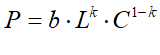
Cobb and Douglas found that result by fitting the function shown in Equation to index number data, which they had laboriously assembled from Census data and an established index of manufacturing output (see Table 4 in the Appendix). In Equation , P stands for manufacturing output, L and C for employment and capital respectively in manufacturing, and b is a constant:
Their regression returned the result shown in Equation :
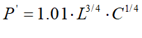
They reported an extremely high correlation coefficient, not merely for Equation , but for what they described as the data “with trends eliminated”:
The coefficient of correlation between P
and P’ with trends included is .97 and with trends eliminated is .94. (Cobb and Douglas 1928, p. 154)
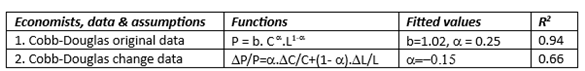
This implied a high level of robustness for their result, but this is not the case. The results and high correlations for the absolute value data are correct, but as Samuelson later observed, this was largely due to the collinearity of the data (Samuelson 1979, pp. 929). However, their stated results for the “trends eliminated” data are an artefact of their method of de-trending, which was to analyse the three-year moving average. When annual changes are used, the results are disastrous: the coefficient for is negative (and, for what it’s worth, the R2 is much lower)—see Table 1.
Table 1: Parameter values and R2 from the Cobb-Douglas index data, and annual fractional change in the data
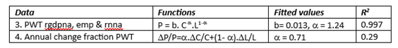
The results are similarly bad when modern data is fitted—see Table 5 in the Appendix for the Penn World Tables data for the USA from 1950 till 2019 (Feenstra, Inklaar, and Timmer 2015) and the fractional annual rate of change. The results from fitting the CDPF to this data are shown in Table 2 and are similarly disastrous for Neoclassical theory. A fit of the CDPF to aggregate data returns an of 1.24, which heavily weights Capital’s contribution to output, and gives Labour a negative weight. The annual rates of change data generates a value for which is less than 1, but also “wrong”, in terms of the Neoclassical theory of income distribution: it attributes 71% of the change in output to Capital and only 29% to Labour. This may in fact be more realistic, but it conflicts with distribution of income data, and therefore with Neoclassical theory. As Solow said, had Cobb and Douglas returned results like these, Neoclassical economists “would not now be discussing aggregate production functions”.
Table 2: CDPF fitted to PWT data for the USA from 1950 till 2019
Rescued by Solow’s Residual
However, Neoclassical economists were saved the embarrassment of encountering these results by Solow’s introduction of technical change into the CDPF. His intentions were laudable, but to achieve his objective he had to add two assumptions—that the exponents in the CDPF were the marginal products of Labour and Capital, and that these were equivalent to income-share data:
The new wrinkle I want to describe is an elementary way of segregating variations in output per head due to technical change from those due to changes in the availability of capital per head. Naturally, every additional bit of information has its price. In this case the price consists of one new required time series, the share of labor or property in total income, and one new assumption, that factors are paid their marginal products. Since the former is probably more respectable than the other data I shall use, and since the latter is an assumption often made, the price may not be unreasonably high. (Solow 1957, p. 312. Emphasis added)
Of course, Neoclassical economists were more than willing to pay this “price”, since it was to assume that their theory of production and of income distribution were both correct, and consistent with each other. They could then derive the contribution of change in technology from the difference between change in GDP and change in the two income-distribution-weighted “factors of production”. From this date on, the exponents in the CDPF were not derived from empirical data, but were simply assumed to be correct, and equal to the shares of Labour and Capital in income distribution data—1/3rd for Capital and 2/3rds for Labour (Solow 1957, Table 1, p. 315). Variation between changes in output and the weighted changes in inputs was attributed to “total factor productivity” and measured by “the Solow Residual”. The fact that, in Solow’s initial paper, 87.5% of growth was attributed to technical change, and only 12.5% to changes in the factor proportions of Labour and Capital, was only moderately embarrassing. Subsequently, Neoclassical economists have since simply assumed that their models of production and distribution are correct, and the coefficients of the CDPF have altered from flawed empirical findings to unquestioned theoretical assumptions.
All of this was without considering energy: to this day, the vast majority of Neoclassical models of production consider only Labour and Capital as inputs. But when energy was considered by some Neoclassicals, it was accorded the same treatment: its exponent was set by its share in GDP, and this was assumed to be equal to its marginal productivity.
The Power(lessness) of Energy?
Two of the very few Neoclassical papers that include energy in a production function and ascribe a numerical value to it are (Engström and Gars 2016) and (Bachmann et al. 2022). The former uses an exponent of 0.03 and the latter of 0.04, in production functions of the form shown in Equation :
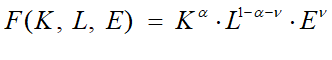
Both made Solow’s assumption that the share of energy in GDP is equal to the marginal productivity of Energy. This led Bachmann et al. to comment that:
Therefore, for example, a drop in energy supply of log E = -10% reduces production by logY = 0.04 x 0.1 = 0.004 =0.4% … [which] … “shows that production is quite insensitive to energy E as expected” (Bachmann et al. 2022, Appendix, p. 5. Emphasis added).
The data begs to differ. Table 6 and Figure 1 to Figure 5 show Gross World Product against Primary Energy Supply for the years 1971 till 2019. Far from production being “quite insensitive to energy”, as assumed by Neoclassical economists, the empirically derived value of  is 0.97, rather than the 0.03-0.04 value assumed by Neoclassical economists. Instead of production being “quite insensitive to energy”, to a reasonable first approximation, production is Energy.
Table 3 shows the coefficients for regressing GDP and change in GDP |(Y/Y) against linear equations for Energy and change in Energy (E/E).
Table 3: Regression of Energy against Gross World Product
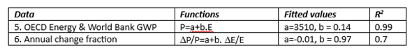
Figure 1: Gross World Product and Energy Consumption over time
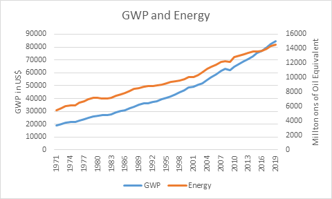
Figure 2: Energy vs GWP
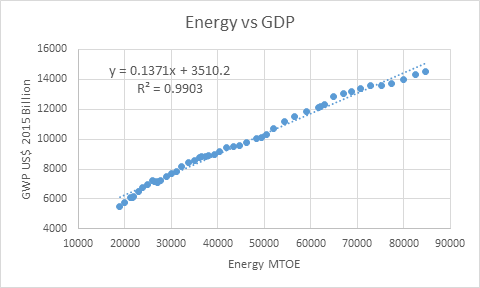
Figure 3: Ratio of GWP in US$2015 billion to Energy in MTOE from 1971 till 2019
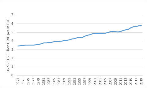
Figure 4: Change in GWP and Change in Energy in Percent p.a.
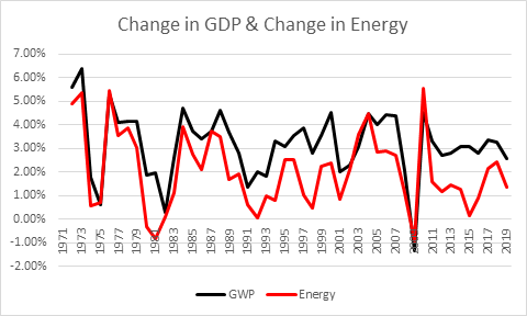
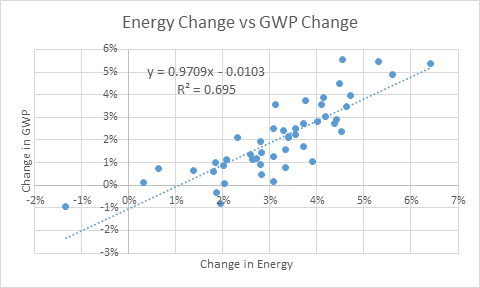
Figure 5: Correlation of change in Energy and change in GWP in Percent p.a.
This empirical data, as Bachmann et al. unintentionally show, is an effective refutation of the Neoclassical theories of production and income distribution, and confirmation of the Post-Keynesian theories.
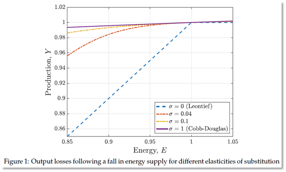
They compare the polar opposites of the Cobb-Douglas and the Leontief in a CES production function, where the elasticity of substitution between inputs for Cobb-Douglas equals 1 and that for Leontief equals 0. They correctly lay out the implications of the Leontief case, that:
Leontief production… implies that Y = E/ … and hence logY = log E … Therefore, if the elasticity of substitution is exactly zero, production Y drops one-for-one with energy supply E … Intuitively, the Leontief assumption means that energy is an extreme bottleneck in production: when energy supply falls by 10%, the same fraction 10% of the other factors of production X lose all their value (their marginal product drops to zero) and hence production Y falls by 10%. (Bachmann et al. 2022, Appendix, pp. 5-6. Emphasis added)
They plotted the theoretical relationships between energy input and GDP output for different values of the substitution parameter in their Figure 1 (reproduced as Figure 6 here).
Figure 6: Bachmann et al.’s theoretical predictions of change in output for a change in energy
They then rejected the Leontief function, on the grounds that its prediction of a 1:1 fall in production for a fall in energy leads to nonsensical results in terms of Neoclassical theory:
Extreme scenarios with low elasticities of substitution and why Leontief production
at the macro level is nonsensical … The blue dashed line in Figure 1 showed that output falls one-for-one with energy supply in the Leontief case… the marginal product of energy jumps to 1/ [their exponent for energy] while the marginal product of other factors … falls to zero. If … factor prices equal marginal products, this then implies that similarly the price of energy jumps to 1/ and the prices of other factors a fall to zero… this then also implies that the expenditure share on energy jumps to 100% whereas the expenditure share on other factors falls to 0%. We consider these predictions to be economically nonsensical. (Bachmann et al. 2022, p. 15. Italicised emphasis added)
These predictions are nonsensical, but at the same time, the Leontief case fits the empirical data (which, following Solow’s lead, they did not consult). It is not the data which is false, but the assumption they made that “factor prices equal marginal products”. Therefore, wages, profits and the price of energy cannot be based upon the “marginal product” of labour, capital and energy respectively. The Neoclassical Cobb-Douglas model of production is false, and the Post-Keynesian Leontief model of production is correct. The question now remains as to why the Leontief model is correct.
From Empirical Regularity to the Role of Energy in Production
The Leontief Production Function began as an empirical regularity between GDP, however measured, and Capital, however measured. The ratio was relatively constant over time and showed no trend—see Figure 7 for Capital to Output ratios derived from the Penn World Tables database.
Figure 7: Capital to Output Ratios are reasonably constant over time
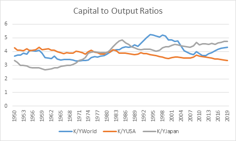
This led to the pragmatic Post-Keynesian school adopting the capital to output ratio as its “production function”, with the justification that this relationship was found in the data, but with no real explanation as to why it was found. Leaving aside the minimum form in which the LPF is often expressed but seldom used, we have, as in the Goodwin model (Goodwin 1967):

Here v is the capital to output ratio. With K having the dimension of Widgets, and Y of Widgets per year, for dimensional accuracy, v must be a time constant denominated in Years.
The empirical regularity behind the LPF can be explained by the aphorism that Ayres, Standish and I applied in “A Note on the Role of Energy in Production” (Keen, Ayres, and Standish 2019), that:
labour without energy is a corpse, while capital without energy is a sculpture. (Keen, Ayres, and Standish 2019):
This suggested that the inputs of Labour and Capital assumed by both the CDPF and the LPF should be replaced by the energy inputs to both Labour and Capital, via the substitution shown in Equation :
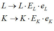
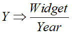
Here respectively L and K stand for units of Labour and Capital, EL and EK represent the energy consumed by a unit of Labour and a unit of Capital, and eL and eK are time constants (dimensioned by 1/Year) representing the proportion of these inputs that are turned into useful work over a Year. This then suggests a way to derive the LPF from the dimensionality of the substitution proposed in Equation (5). In the standard single commodity CDPF and LPF, Y and K are denominated in “widgets per year” and “widgets” respectively—units of a universal commodity that can be used for either investment or consumption:
The substitution in (5) on the other hand has the dimensionality of units of Energy per year:
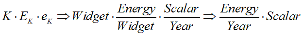
Call this Q, denominated in units of Energy per year, to distinguish it from Y, denominated in units of widgets per year:
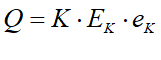
Y is therefore equal to Q divided by EK:
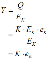
Equating Equation (9) with Equation (4) shows that the empirically derived capital to output ratio v is in fact the inverse of the proportion of inputted energy that machinery turns into useful work:
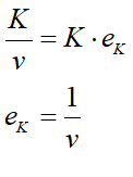
This provides a physical explanation for the empirical regularity on which the Post-Keynesian model of production is based: it is due to the role of machinery in turning energy—predominantly fossil fuel energy—into useful work. This model therefore ties Post-Keynesian theory to the initial accurate insights of the Physiocrats, that Nature is the source of wealth, and that what human ingenuity does is enable the conversion of “this superfluity that nature accords him as a pure gift” (Turgot 1774, p. 9) into useful work. Given the close relationship between GDP and Energy shown in Figure 2 to Figure 5, at a first approximation, GDP is useful energy. Equation (9) can therefore be used in place of Equation (4) in Post-Keynesian models.
The Post-Keynesian model is also consistent with the Laws of Thermodynamics, including the Second Law (which the Physiocrats did not realise) that doing work generates waste as well as desired output. With the capital to output ratio averaging 4 globally, and ranging between 3 and 5 for developed nations, the magnitude of eK is of the order of 0.2-0.33. This then quantifies the waste generated in production as being of the order of 0.67-0.8: humanity generates more waste than output. The constancy of the capital to output ratio, much criticised by Neoclassical economists, is in fact due to the impossibility of substituting any other input for energy, and intrinsic limits to the efficiency of conversion of energy into useful work given by the Second Law of Thermodynamics.
Conclusion
The Neoclassical Cobb-Douglas Production Function, with its exponents assumed to be equal to the income shares of factor inputs, and also equal to the marginal product of those inputs, cannot be reconciled with energy data, or with the Laws of Thermodynamics, and it is therefore wrong.
The Post-Keynesian Leontief Production Function, on the other hand, is not only empirically accurate, but is also consistent with the Laws of Thermodynamics. Though the construction of a universal commodity in aggregate production functions has always been a convenience, the fact that GDP and Energy are so tightly coupled means that the LPF is a reasonable first approximation to reality. Solow’s observation that “As long as we insist on practicing macroeconomics we shall need aggregate relationships” (Solow 1957, p. 213) is correct, but the only aggregate production function that fits the bill is the Leontief Production Function.
Bachmann, Rüdiger, David Baqaee, Christian Bayer, Moritz Kuhn, Andreas Löschel, Benjamin Moll, Andreas Peichl, Karen Pittel, and Moritz Schularick. 2022. ‘Was wäre, wenn…? Die wirtschaftlichen Auswirkungen eines Importstopps russischer Energie auf Deutschland; What if? The macroeconomic and distributional effects for Germany of a stop of energy imports from Russia’, ifo Schnelldienst, 75.
Cantillon, Richard. 1755. Essay on Economic Theory (Ludwig von Mises Institute).
Cobb, Charles W., and Paul H. Douglas. 1928. ‘A Theory of Production’, The American Economic Review, 18: 139-65.
Eddington, Arthur Stanley. 1928. The Nature Of The Physical World (Cambridge University Press: Cambridge).
Engström, Gustav, and Johan Gars. 2016. ‘Climatic Tipping Points and Optimal Fossil-Fuel Use’, Environmental and Resource Economics, 65: 541-71.
Feenstra, Robert C., Robert Inklaar, and Marcel P. Timmer. 2015. ‘The Next Generation of the Penn World Table’, American Economic Review, 105: 3150-82.
Felipe, J., and J. S. L. McCombie. 2014. ‘The Aggregate Production Function: ‘Not Even Wrong”, Review of Political Economy, 26: 60-84.
Felipe, Jesus, and John McCombie. 2011. ‘On Herbert Simon’s criticisms of the Cobb-Douglas and the CES production functions’, Journal of Post Keynesian Economics, 34: 275-94.
———. 2020. ‘The illusions of calculating total factor productivity and testing growth models: from Cobb-Douglas to Solow and Romer’, Journal of Post Keynesian Economics, 43: 470-513.
Felipe, Jesus, and John S. L. McCombie. 2007. ‘Is a Theory of Total Factor Productivity Really Needed?’, Metroeconomica, 58: 195-229.
Fisher, Franklin M. 1971. ‘Aggregate Production Functions and the Explanation of Wages: A Simulation Experiment’, The Review of Economics and Statistics, 53: 305.
Georgescu-Roegen, Nicholas. 1993. ‘Thermodynamics and We, the Humans.’ in J. C. Dragan, E. K. Seifert and M. C. Demetrescu (eds.), Entropy and bioeconomics: Proceedings of the First International Conference of the European Association for Bioeconomic Studies, Rome 28-30, November 1991 (Nagard: Milan).
Goodwin, Richard M. 1967. ‘A growth cycle.’ in C. H. Feinstein (ed.), Socialism, Capitalism and Economic Growth (Cambridge University Press: Cambridge).
Harcourt, G. C. 1972. Some Cambridge Controversies in the Theory of Capital (Cambridge University Press: Cambridge).
Keen, Steve, Robert U. Ayres, and Russell Standish. 2019. ‘A Note on the Role of Energy in Production’, Ecological Economics, 157: 40-46.
Marshall, Alfred. 1890 [1920]. Principles of Economics ( Library of Economics and Liberty).
McCombie, John S. L. 2000. ‘The Solow Residual, Technical Change, and Aggregate Production Functions’, Journal of Post Keynesian Economics, 23: 267-97.
———. 2001. ‘Reflections on Economic Paradigms and Controversies in Economics’, Zagreb International Review of Economics and Business, 4: 1-25.
Samuelson, Paul A. 1979. ‘Paul Douglas’s Measurement of Production Functions and Marginal Productivities’, Journal of Political Economy, 87: 923-39.
Shaikh, Anwar. 1974. ‘Laws of Production and Laws of Algebra: The Humbug Production Function’, Review of Economics and Statistics, 56: 115-20.
———. 1980. ‘Laws of production and laws of algebra: Humbug II.’ in Edward J. Nell (ed.), Growth, Profits and Property (Cambridge University Press).
———. 1987. ‘Humbug production function.’ in John Eatwell, Murray Milgate and Peter Newman (eds.), The New Palgrave: A Dictionary of Economics (Palgrave Macmillan).
———. 2005. ‘Nonlinear Dynamics and Pseudo-Production Functions’, Eastern Economic Journal, 31: 447-66.
Smith, Adam. 1776. An Inquiry Into the Nature and Causes of the Wealth of Nations (Liberty Fund: Indianapolis).
Solow, R. M. 1974a. ‘Intergenerational Equity and Exhaustible Resources’, Review of Economic Studies, 41: 29.
Solow, Robert M. 1957. ‘Technical Change and the Aggregate Production Function’, The Review of Economics and Statistics, 39: 312-20.
———. 1974b. ‘The Economics of Resources or the Resources of Economics’, The American Economic Review, 64: 1-14.
Stiglitz, Joseph. 1974a. ‘Growth with Exhaustible Natural Resources: Efficient and Optimal Growth Paths’, The Review of Economic Studies, 41: 123-37.
Stiglitz, Joseph E. 1974b. ‘Growth with Exhaustible Natural Resources: The Competitive Economy’, Review of Economic Studies, 41: 139.
Turgot, Anne Robert Jacques. 1774. Reflections on the Formation and Distribution of Wealth (London: Spragg).
Ulgiati, Sergio, and Carlo Bianciardi. 2004. ‘Thermodynamics, Laws of.’ in J. Cleveland Editor-in-Chief: Cutler (ed.), Encyclopedia of Energy (Elsevier: New York).