The macro commentator Alfonso Peccatiello, who writes as @MacroAlf on Twitter/X and publishes the Macro Compass newsletter, recently posted an excellent thread on private debt that cited my work:
Let me show you one of the most underrated and yet crucial long-term macro variables in the world. Debt. But not government debt: people should stop obsessing it! The government can print money in its own currency. Of course, this has limitations: capacity constraints, inflation, credibility…but there is much more vulnerable source of debt out there. Private sector debt levels and trends are by far a more important macro variable to follow.
Let me explain why. The private sector doesn’t have the luxury to print money: if you get indebted to your eyeballs and you lose your ability to generate income, the pain is real. This amazing chart from my friend @darioperkins proves the point quite eloquently…
Figure 1: Alf’s chart of private debt to GDP bubble for 4 key economies
This post follows up on Alf’s lead by producing a private debt-focused profile of all the major economies in the OECD whose debt levels are also recorded by the Bank of International Settlements. It combines data on inflation and unemployment rates from the OECD with private and government debt and house price data from the BIS.
The plots in this post run in reverse alphabetical order from the United States (see Figure 2) to Australia. Their message is the same that Alf made in his tweet stream (x-stream?): private debt matters, and the fact that conventional Neoclassical economics ignores it is a major reason why it has failed as a guide to economic theory and policy.
This post also showcases Ravel©™, a multidimensional analytic database which I have designed, and which Minsky’s programmer Dr Russell Standish has coded. We hope to release Ravel commercially in 2024. If you like what you see here, then let me know in the comments and I’ll add you to the early pre-release of Ravel, which we hope will occur in early 2024 (comments are only open to paid subscribers on Patreon and Substack). The end of the post will briefly explain how the plots were created.
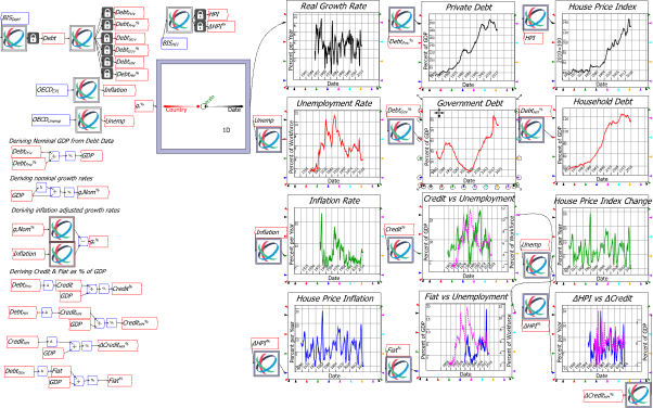
Figure 2: The USA’s data
Several common themes turn up in almost all countries in these plots. First and foremost, the shift from so-called “Keynesian” to “Neoclassical/Neoliberal” economic policies that began in the mid-1970s, which was supposed to unleash the private sector from the shackles of the State, has failed on its own terms. The rate of economic growth under Neoliberalism—which I date from the beginning of 1975, when a surge in inflation empowered the political and academic rise of Milton Friedman’s “Monetarism”—has been lower for every country in this database. Rather than the Neoclassicals showing the Keynesians how to promote growth, the Neoclassicals have shown how to turn real economic performance into permanent financial speculation:
- The rate of economic growth (top left graph) has trended down over time, and rather than reversing this trend, Neoliberalism has accentuated it.
- The unemployment rate is higher and more volatile than in the “bad old Keynesian days”.
- Neoliberalism might claim the low-inflation period after the GFC as a success story, but even so, post-GFC inflation is higher than the record of the 1960s.
- The average rate of economic growth rate has been substantially lower after the deregulation fetish began than before—at 1.8% p.a. in the USA’s case, the average rate of economic growth since Neoliberalism is barely more than half the 3.25% p.a. from 1945 till 1975.
- The main growth success of the Neoliberal period has been an unprecedented increase in private debt. In America’s case, it has tripled from under 60% of GDP at the end of WWII to a peak of almost 180% during the GFC (Global Financial Crisis).
- Government debt is much lower than private debt, and yet it’s government debt that is the unwarranted focus of economic discussion and policy, as Alf pointed out. Nonetheless, even government debt has risen under Neoliberalism, and in the USA’s case the post-GFC level exceeds the pre-Neoliberal peak. That reducing the ratio of government debt to GDP was even made a (failed) policy target is a sign of how little Neoclassical economists know about the economy, since government debt is in fact a record of fiat money creation.
- By stifling the growth of Fiat money, the Neoliberal period encouraged the growth of Credit—the annual change in private debt. While Neoclassical economists like Ben Bernanke bleat that “pure redistributions [as they falsely characterise new private debt] should have no significant macroeconomic effects” (Bernanke 2000, p. 24), Credit strongly negatively correlates with unemployment: when Credit is high unemployment is low and vice versa. This shows, as Alf argued, that credit is a far more important determinant of economic performance than government spending, and yet mainstream economic theory and policy continue to ignore it.
- Government money creation tends to be driven by the rise and fall of unemployment. Since unemployment in general has risen under Neoliberalism, and economic crises that Neoclassicals thought they had abolished (“macroeconomics in this original sense has succeeded: Its central problem of depression prevention has been solved, for all practical purposes, and has in fact been solved for many decades”: Lucas 2003, p. 1) have become more extreme and frequent, panic rather than policy has driven government spending higher as a proportion of GDP under their misguided guidance.
- House prices were tame before Neoliberalism and have been wild ever since, because the housing market has been the main destination of rising private debt. Though Neoliberal politicians like Reagan and Thatcher, Clinton and Blair, believed they were liberating the private sector in general, what they really did was let the financial sector rip.
- The fuel beneath rising house prices has been rising household debt. This has risen even more than total private debt—in the USA’s case, household debt is now fives times as large as it was at the end of WWII, when compared to GDP.
- Turning housing from a long-term consumption item into a financial commodity has led to house price volatility. Richard Vague’s magisterial survey of the last two centuries of financial crises (Vague 2019) shows that house price bubbles are overwhelmingly the main factor behind financial crises. This is what Neoliberalism really gave us.
- Lastly, there is a causal link between change in the level of new mortgage debt and change in house prices. Since houses are bought primarily with borrowed money, the flow of new mortgages is the main monetary foundation of the existing price level. It follows that change in new mortgages drives change in house prices. Neoliberalism promised economic prosperity, but by its ignorance of money has turned our economies into unstable, private-debt-financed casinos.
The following plots are displayed in Ravel simply by moving the selector dot on the master Ravel in the right-hand corner of the model. Figure 3 to Figure 25 show the same data for other countries, in reverse alphabetical order from the UK to Australia.
Figure 3: UK
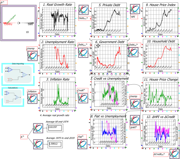
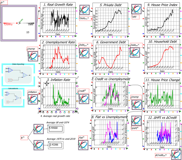
Figure 4: Switzerland
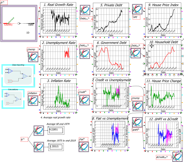
Figure 5: Sweden
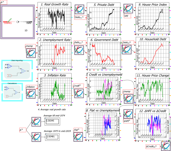
Figure 6: Spain
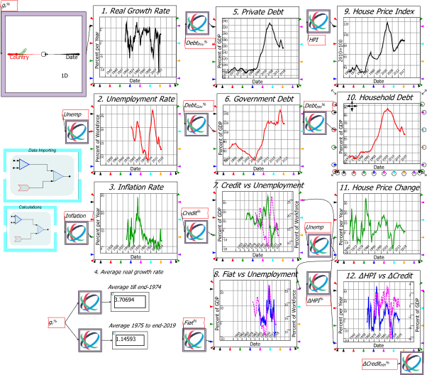
Figure 7: Portugal
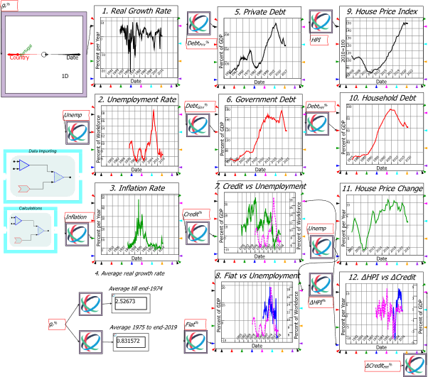
Figure 8: Poland
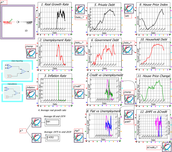
Figure 9: Norway
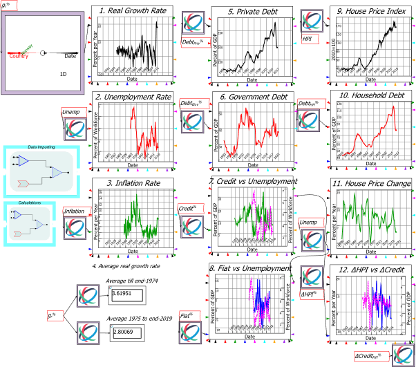
Figure 10: New Zealand
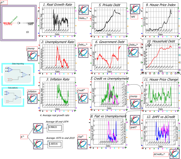
Figure 11: Netherlands
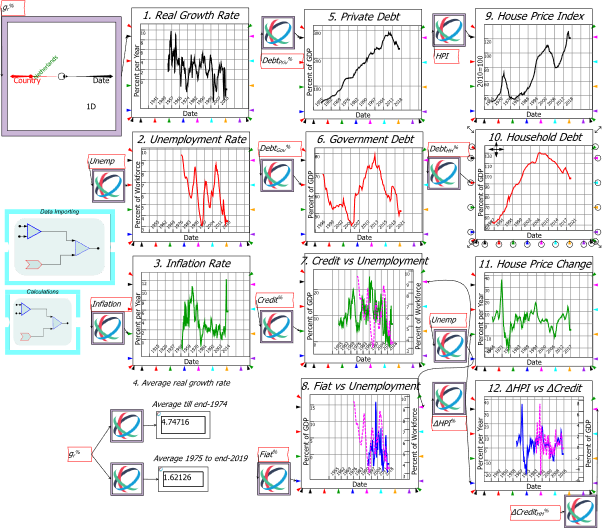
Figure 12: Mexico
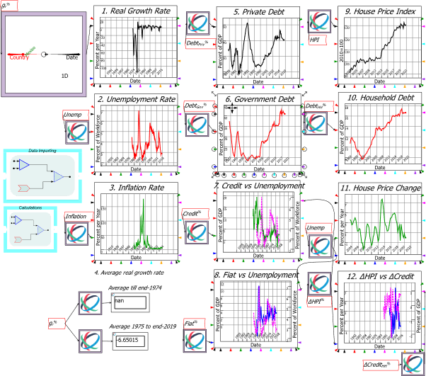
Figure 13: Japan
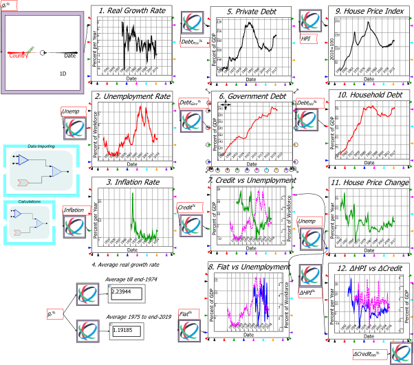
Figure 14: Italy
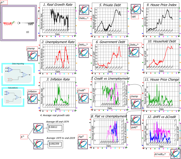
Figure 15: Israel
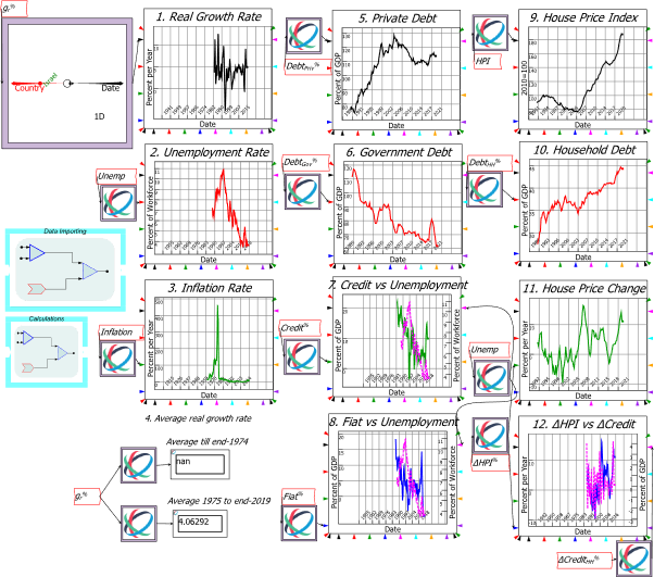
Figure 16: Hungary
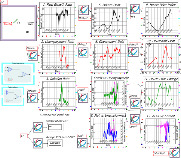
Figure 17: Greece
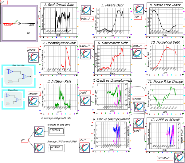
Figure 18: Germany
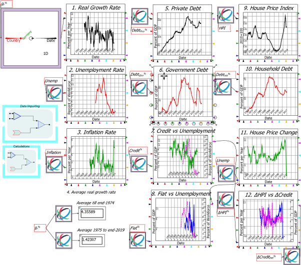
Figure 19: France
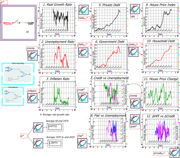
Figure 20: Finland
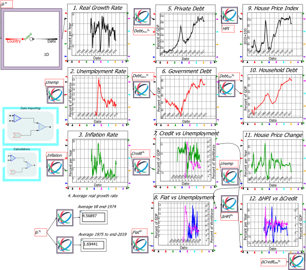
Figure 21: Denmark
Figure 22: Canada
Figure 23: Belgium
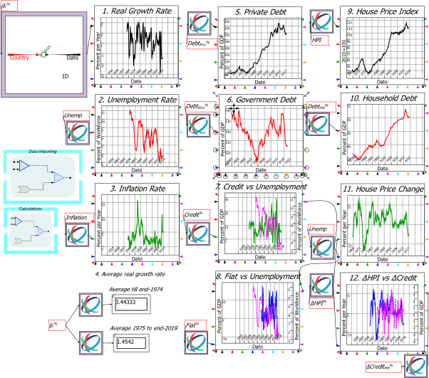
Figure 24: Austria
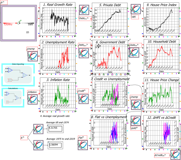
Figure 25: Australia
Using Ravel
The first stage in using Ravel is to import the data, in this case from the BIS and the OECD—which is what Figure 26 illustrates. An importing form specifies which columns in a database are “dimensions” and which are data. At present we only import CSV files, but the range of import formats will grow after the first release.
Figure 26: Data imported into Ravel
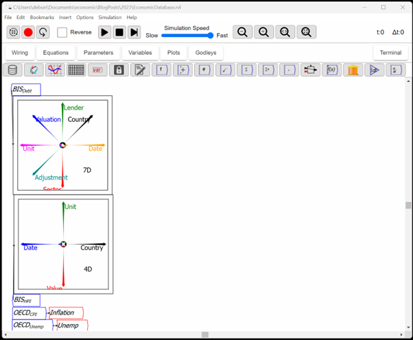
This imported data (stored in the parameters BISDebt, BISHPI, OECDCPI and OECDUnemp) is then, if necessary, attached to a Ravel—the square boxes in Figure 27 with arrows inside them—to enable manipulation of the data and extraction of subsets for further analysis. The top Ravel in Figure 27 stores data on government and private debt in numerous ways—raw domestic currency, percent of GDP, etc. The operations on that Ravel—collapsing one axes and extracting the maximum value stored on it, selecting a single instance (Lending by All Sectors rather than Banks alone, Adjusted for Breaks rather than unadjusted)—reduce a 7-dimensional object to a 4-dimensional one, where those dimensions are Country, Date, Sector, and Unit.
Figure 27: using Ravel’s slice, dice and aggregate functions
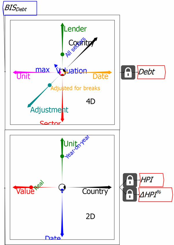
Figure 28 then takes the 4-dimensional object Debt and separates it into Private Debt in domestic currency, private debt as a percentage of GDP, and Government debt as a percentage of GDP.
Figure 28: Minimizing Ravels and selecting slices of debt data
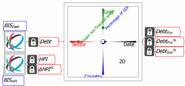
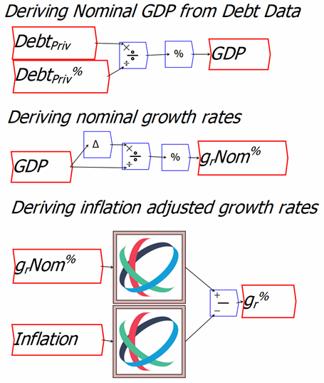
Figure 29 showcases Ravel‘s analytic power, in three ways:
- There is no easily accessible database on quarterly GDP by country, but the BIS database has raw data from which it can be derived. If you divide private debt in domestic currency by private debt as a percentage of GDP, and then multiply that by 100, you have GDP in domestic currency for all the countries in the BIS database. There are over 40 countries and close to 400 quarters of data: that would take 16,000 replicated cell formulas in Excel, but it takes just one flowchart equation in Ravel.
- Nominal growth rate data can be derived by dividing the annual change in GDP by itself and multiplying by 100. Once again, one flowchart formula replaces close to 16,000 Excel formulas; and finally,
- The real growth rate can be derived by subtracting the inflation rate from the nominal growth rate.
Figure 29: Deriving Quarterly nominal GDP and growth rates for the 43 countries in the BIS database
The final database is shown in Figure 30, with one country—Australia, simply because it’s the first alphabetically—highlighted.
Figure 30: The completed economic database
The importing and calculation routines are then put into groups and reduced in size to reduce clutter on the final dashboard used for this document.
References
Bernanke, Ben S. 2000. Essays on the Great Depression (Princeton University Press: Princeton).
Lucas, Robert E., Jr. 2003. ‘Macroeconomic Priorities’, American Economic Review, 93: 1-14.
Vague, Richard. 2019. A Brief History of Doom: Two Hundred Years of Financial Crises (University of Pennsylvania Press: Philadelphia).