An essential component of Neoclassical microeconomics is the proposition that firms maximize their profits by equating marginal revenue—the addition to total revenue caused by the last unit sold—to marginal cost—the addition to total costs caused by the last unit produced. This proposition plays a fundamental role in all DSGE-based macroeconomic models too, in the form of profit maximization rules for the competitive and monopolistic industry sectors that are integral parts of these models. The former maximize profits by setting price equal to marginal cost: since they lack market power, for them, the market price is a constant, and therefore price equals marginal revenue. The latter set price at a markup above marginal cost, at the point where marginal cost equals marginal revenue.
This is chapter five of my draft book Rebuilding Economics from the Top Down, which will be published later this year by the Budapest Centre for Long-Term Sustainability
The previous chapter was The “Anything Goes” Market Demand Curve, which is published here on Patreon and here on Substack.
If you like my work, please consider becoming a paid subscriber from as little as $10 a year on Patreon, or $5 a month on Substack
The formulas in DSGE models that apply these rules are normally far more complicated than the simple rules taught in microeconomic textbooks, but they are based on the same principles: setting marginal revenue equal to marginal cost maximizes profits, because these are the slopes respectively of total revenue and total cost. When the slopes of the total revenue and total cost curves are the same, the gap between them—which is total profit—is maximized.
There are logical problems with this argument (Keen and Standish 2010, 2015), but there is a far more important problem: the conclusion that a firm maximises profits by equating marginal revenue and marginal cost requires that marginal cost rises with output, but this condition does not apply for the vast majority of firms in the real world.
The logical basis of the condition is the “The Law of Diminishing Returns”, that output rises as variable inputs rise, but at a decreasing pace. To cite Samuelson and Nordhaus’s textbook again:
Under the law of diminishing returns, a firm will get less and less extra output when it adds additional units of an input while holding other inputs fixed. In other words, the marginal product of each unit of input will decline as the amount of that input increases, holding all other inputs constant. (Samuelson and Nordhaus 2010, pp. 108-109)
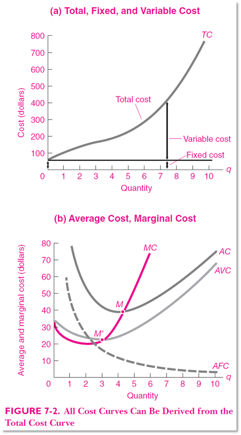
The Law of Diminishing Returns then generates the standard model of a firm’s cost structure, in which marginal costs are steeply rising, the average total cost curve is U-shaped, and average fixed costs are relatively small—see Figure 5, which is taken from Samuelson and Nordhaus’s textbook.
Figure 5: The standard textbook model of the cost structure of the representative firm (Samuelson and Nordhaus 2010, p. 131)
The Law of Diminishing Returns is logically correct, given its assumptions, as is the shape of the cost curves derived from it. But it is also, to quote the humourist H. L. Mencken, “neat, plausible, and wrong”. When economists have investigated the actual cost structures of real firms—as opposed to the imaginary ones with which economics textbooks are populated—the universal result has been that, for the vast majority of firms, marginal cost is either constant, or falls with increasing output.
The last economist to discover this was Alan Blinder, who ranks as highly as Blanchard in the pantheon of influential Neoclassical economists: he was Vice-Chair of the Federal Reserve, Vice-President of the American Economic Association, and was and remains a prominent “New Keynesian” macroeconomist.
A distinguishing feature of “New Keynesian” DSGE models, compared to “New Classical” RBC (“Real Business Cycle”) models, is that New Classicals assume that prices adjust instantly to clear markets, whereas New Keynesians assume that prices are “sticky”—and hence that some unemployment of resources is involuntary. New Keynesians came up with many theories as to why prices should be sticky, each with different implications for the economy. To resolve this debate, Blinder decided to do a survey of American manufacturing firms, to see if their prices were indeed “sticky”, and if so, why.
The survey itself was enormous: 200 firms were directly interviewed, and their output accounted for “7.6 percent of the total value added in the nonfarm, for-profit, unregulated sector” of the US economy (Blinder 1998, p. 67). It was, without a doubt, the largest survey ever undertaken of the cost structures and behaviours of corporations.
It also contained a surprise for Neoclassical economists, which Blinder introduced as follows:
Another very common assumption of economic theory is that marginal cost is rising. This notion is enshrined in every textbook and employed in most economic models. It is the foundation of the upward-sloping supply curve…
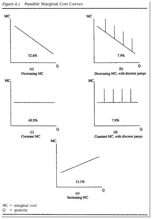
The overwhelmingly bad news here (for economic theory) is that, apparently, only 11 percent of GDP is produced under conditions of rising marginal cost. Almost half is produced under constant MC … But that leaves a stunning 40 percent of GDP in firms that report declining MC functions. (Blinder 1998, pp. 101-102. Emphasis added)
Blinder summarised this result in what is possibly the ugliest graph ever published in an economics book—see Figure 6.
Figure 6: Blinder’s graphical summary of his survey’s findings on the shape of the marginal cost curve
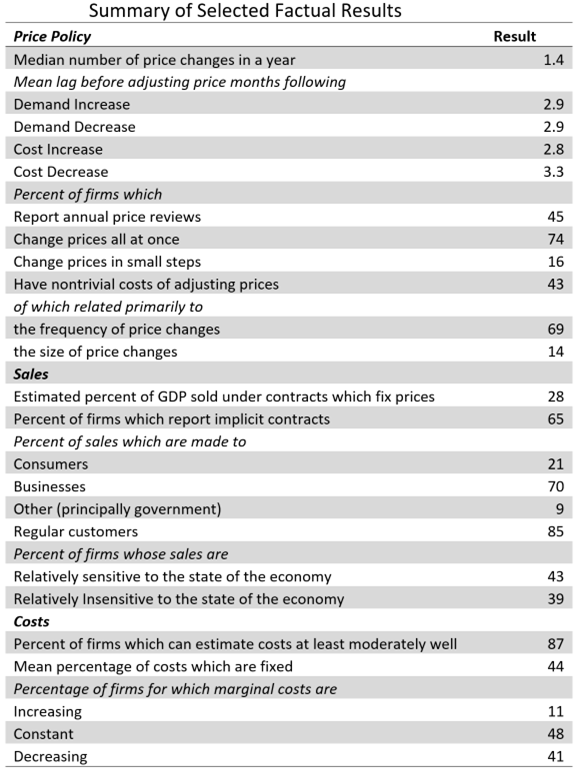
In fact, virtually all of Blinder’s empirical findings were a surprise to Neoclassical economists. For my purposes here, the second-largest surprise (after the discovery that marginal costs are either constant or falling) was that average fixed costs were extremely high—compared to conventional economic theory—at on average 44% of average total costs at the firm’s normal operating level (see Table 1). Compare that to Samuelson and Nordhaus’s toy model in Figure 5, where average fixed costs are far smaller than average variable and marginal costs. [Footnote 1]
Table 1: Blinder’s summary of his empirical results (Blinder 1998, p. 106)
Blinded concluded that:
While there are reasons to wonder whether respondents interpreted these questions about costs correctly, their answers paint an image of the cost structure of the typical firm that is very different from the one immortalized in textbooks. (Blinder 1998, p. 105. Emphasis added)
However, though these results were a surprise to textbook writers, they were not at all a surprise to anyone who had ever surveyed firms about their cost structures. The definitive survey of such surveys was done by Fred Lee (Lee 1998). He found 71 surveys between 1924 and 1979, all of which found the same result, that marginal costs are constant or falling for the vast majority of firms.
The definitive explanation for this phenomenon—which contradicts the “Law” of Diminishing Returns—was given by Andrews in 1949:
On the usual assumptions, the static law of diminishing returns is held to justify the short-run average-cost curve being drawn as U-shaped. The rising branch of the U, in particular, is justified by the assumption that there will be an optimum dosage of the direct [“variable costs”] cost factors, after which average direct costs rise and, in the end, more than counterbalance the effect of the falling overhead-cost curve [“fixed costs”].
However, the rising part of the average direct-cost curve, and hence of the average total-cost curve, even when it would exist, is not relevant to normal analysis. The normal situation is that the businessman will plan to have reserve capacity, his average-cost curve falling for any outputs that he is likely to meet in practice, and his average direct costs, which the second part of this paper will treat as of crucial importance in the theory of pricing, normally being practically constant for very wide ranges of output. (Andrews, Lee, and Earl 1993, p. 78; Andrews 1949)
The reasons why real-world firms have substantial excess capacity, and therefore do not experience diminishing marginal productivity, are quite simple.
Firstly, Neoclassical textbooks describe factories as cartoonish shambles. For example, this is Mankiw’s explanation of why “Hungry Helen’s Cookie Factory” experiences diminishing marginal productivity:
At first, when only a few workers are hired, they have easy access to Helen’s kitchen equipment. As the number of workers increases, additional workers have to share equipment and work in more crowded conditions. Hence, as more and more workers are hired, each additional worker contributes less to the production of cookies…
when Helen’s kitchen gets crowded, each additional worker adds less to the production of cookies; this property of diminishing marginal product is reflected in the flattening of the production function as the number of workers rises… Because her kitchen is already crowded, producing an additional cookie is quite costly. Thus, as the quantity produced rises, the total-cost curve becomes steeper. (Mankiw 2001, pp. 273, 275)
“Hungry Helen’s Cookie Factory” is, of course, a made-up example: there is no such firm. Nor does “Thirsty Thelma’s Lemonade Stand” exist, nor “Big Bob’s Bagel Bin”: they are all simply products of Mankiw’s febrile (and alliterative) Neoclassical imagination. Equally, “Al’s Building Contractors” is a fictional example that Blinder uses in his textbook (Baumol and Blinder 2011). [Footnote 2]
In the real world, factories are designed by engineers to reach peak performance at or very near capacity. As Eiteman put it in 1947, engineers design factories:
so as to cause the variable factor to be used most efficiently when the plant is operated close to capacity. Under such conditions an average variable cost curve declines steadily until the point of capacity output is reached. A marginal curve derived from such an average cost curve lies below the average curve at all scales of operation short of peak production, a fact that makes it physically impossible for an enterprise to determine a scale of operations by equating marginal cost and marginal revenues unless demand is extremely inelastic. (Eiteman 1947, p. 913)
Real-world manufacturers, when they had the Neoclassical model explained to them, have often felt insulted by it. For example, Eiteman and Guthrie sent a survey to one thousand firms, which asked them to nominate which of 8 curves most closely approximated their average costs (Eiteman and Guthrie 1952)—see Figure 7. Of the 366 firms who replied, literally only one selected Curve 3, which is the one that is most like the standard drawing in Neoclassical textbooks (such as that in Figure 5 on page 1, from (Samuelson and Nordhaus 2010))—see Table 2. On the other hand, over 60% of firms chose Curve 7, and another 34% chose the very similar Curve 6.
Figure 7: Eiteman & Guthrie’s eight hypothetical average total cost curves (Eiteman and Guthrie 1952, pp. 834-835)
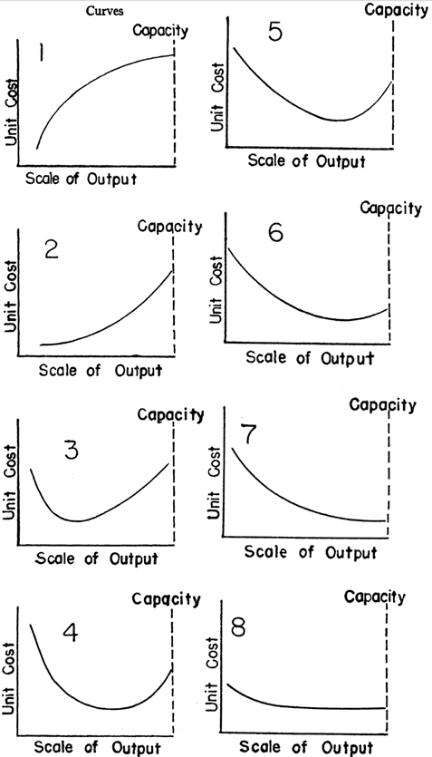
Table 2: The responses to Eiteman and Guthrie’s survey on the shape of the average cost curve: “Table II.-Choice of Cost Curve by Companies Without Reference to Number of Products” (Eiteman and Guthrie 1952, p. 837)
| Curve Indicated |
Number of Companies |
Percent |
| 1 |
0 |
0.0% |
| 2 |
0 |
0.0% |
| 3 |
1 |
0.3% |
| 4 |
3 |
0.9% |
| 5 |
14 |
4.2% |
| 6 |
113 |
33.8% |
| 7 |
203 |
60.8% |
| 8 |
0 |
0.0% |
| Total |
334 |
100.0% |
Eiteman and Guthrie noted that “The replies demonstrate a clear preference of businessmen for curves which do not offer great support to the argument of marginal theorists,” and continued that “If some of the personal comments of those who answered the questionnaires were to be repeated here, they would serve further to emphasize this conclusion”. They cited one businessman, who remarked that:
“‘The amazing thing is that any sane economist could consider No. 3, No. 4 and No. 5 curves as representing business thinking. It looks as if some economists, assuming as a premise that business is not progressive, are trying to prove the premise by suggesting curves like Nos. 3, 4, and 5.” (Eiteman and Guthrie 1952, p. 838)
Secondly, when a factory is first constructed, it is built with expansion of sales in mind: a factory which operates at 100% capacity on day one of its operations is a factory that was too small in the first place.
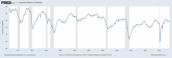
Thirdly, in a genuinely competitive industry, virtually every firm hopes to increase its market share—and precisely because this will increase its profits. It needs spare capacity in order to do this, and since all firms do it, the aggregate potential output of the industry substantially exceeds the proportion that is used. Even during the boom years of the 1960s, capacity utilization in the American economy never exceeded 90%, and it has trended down ever since—see Figure 8.
Figure 8: Aggregate capacity utilization in the USA: https://fred.stlouisfed.org/series/TCU#
The preconditions needed for diminishing marginal productivity to apply therefore do not exist in the real world. They exist only in the childish imaginations of Neoclassical textbook writers.
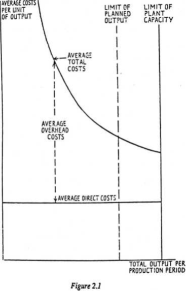
In 1949, Andrews sketched the standard real-world situation, in which diminishing marginal productivity does not apply, because a well-managed firm has idle capacity. Rather than having its machinery operated at beyond its optimal variable inputs to fixed capital ratio, as is assumed by economics textbooks, it has substantial spare capacity.
Figure 9: Andrews’ graphical summary of the normal cost curves for a manufacturing business (Andrews, Lee, and Earl 1993, p. 80)
The practical import of this actual representative shape of the cost curves for a manufacturing firm was given by Eiteman in 1948:
marginal cost curves will lie below average cost curves at all points of operation short of capacity. As a consequence, marginal cost curves will no longer intersect marginal revenue curves (1) when average revenue curves are horizontal or (2) when average revenue curves are high and almost horizontal. Under either of these conditions, business managers would simply produce as much goods as the current market would absorb without reference to marginal cost and marginal revenue. (Eiteman 1948, P. 900. Emphasis added)
The import of this is devastating for both Neoclassical micro and macroeconomics.
Neoclassical microeconomics is predicated on the output level of the firm being based on its marginal cost. A profit-maximizing firm produces where marginal cost equals marginal revenue, because that output level maximizes profits: any higher output level than that actually reduces profits. But as Figure 10 illustrates, marginal cost (which equals variable cost when it is a constant with respect to output) lies well below total cost: any firm that did price at marginal cost would rapidly go bankrupt. The real-world profit-maximization condition is to sell as many units as possible—and preferably at the expense of sales to your rivals, with whom you compete not on price but on non-price issues like product differentiation. Hence, Figure 10 shows price P as a constant, not because of a silly Neoclassical assumption like “perfect information”, but because in a mature industry in the real world, additional sales by one competitor normally come at the expense of the sales by another.
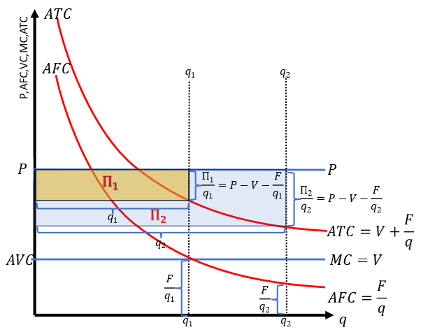
Additional output lowers average fixed costs, which are a very significant component of total costs. Lower per unit fixed costs, with constant per unit variable costs and—in a competitive industry where non-price, product-differentiation-based competition dominates—this results in rising total and per-unit profits as capacity utilization rises, right out to the factory’s capacity, as Figure 10 illustrates.
Figure 10: Profit, Revenue and Costs at the target output level for the representative firm
Real-world profit maximization, therefore, involves selling as many units as possible, rather than stopping selling when “marginal cost exceeds marginal revenue”. Any real-world sales manager who told his staff to stop selling would (and should) be sacked.
This is why Blinder described the results of his survey as “overwhelmingly bad news … (for economic theory)”. Not only does the theory not describe the behaviour of real-world firms, but all the welfare conclusions that flow from marginal this equalling marginal that disappear as well—and they have already been destroyed in any case by the logical fallacies in the derivation of the market demand curve covered in the previous chapter.
Macroeconomics that is based on Neoclassical microeconomics inherits these false microeconomic assumptions, and they play critical roles in the algebraic derivation of an RBC or DSGE model. But in the real world, which these models purport to describe, these conditions are strongly violated.
Therefore, even if it were possible to derive macroeconomics from microeconomics—which the previous chapter showed was a fool’s errand for any complex system—then Neoclassical microeconomics is not the right foundation for it.
So, what to do? I’ll give my alternative in the following chapters, after a brief Appendix which lays out the mathematics of real-world profit maximization, and speculates about what a real-world microeconomics might look like.
-
Appendix: Real World Profit Maximization and Real-World Microeconomics
Eiteman’s conjecture—that the profit-maximisation strategy of real-world firms is to sell as many units as possible—is easily illustrated using Figure 10. A firm with the cost structure of a typical real-world firm has fixed costs of F (which are a substantial component of total costs at the target output level—of the order of 40% of the market price, according to Blinder’s research), constant variable costs per unit AVC=V—so that marginal costs are also constant, and equal to V—total revenue which is equal to the market price P times the quantity sold, and a price level P that substantially exceeds average variable and hence marginal costs: P>V.
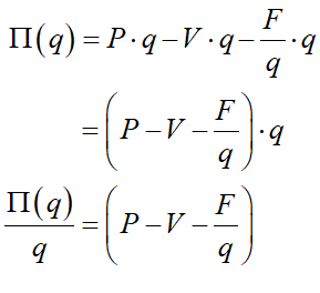
The profits of the firm are given by Equation :
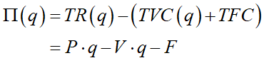
The differential of profit with respect to the quantity sold is therefore always positive:
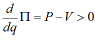
Therefore, as Eiteman said, the best strategy for the firm is to sell as many units as it can. Since its competitors are all trying to do the same thing, while market demand is, for mature industries, a relatively stable fraction of GDP, this leads to the evolutionary competitive struggle we witness in most real-world markets.
We can get a slightly more informative formula by rearranging Equation to show profit per unit:
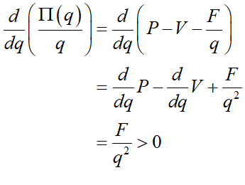
The differential of profit per unit with respect to q is:
The rate of change of profit with respect to output can also be expressed in terms of fixed cost and profit per unit of output by simply rearranging the definition of profit:
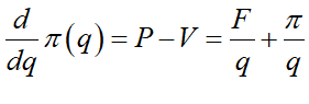
This confirms the graphical intuition in Figure 10. An increase in output means that the height of the rectangle for total fixed costs falls, while the height of the rectangle for total variable costs remains constant, as does the height of the rectangle for total revenue. The falling height of average fixed costs means that the gap between average revenue and average costs grows. Total profit therefore rises with rising output, because the substantial fixed costs of production are spread over a larger number of units sold. Profit per unit grows as fixed costs per unit shrinks.
Given these fundamental problems with both the theory of demand and the model of production, the only thing one can say in favour of Neoclassical microeconomics is that it gives Neoclassical microeconomists something to do. But it is worse than useless in the real world: with of the order of 95% of firms not having the pre-conditions to experience diminishing marginal productivity, and a theory of demand that does not transcend a single individual, the games Neoclassical microeconomists play are just that: games.
This real-world analysis raises the possibility of an evolutionary microeconomics that, while it could not be used to derive macroeconomics, would be compatible with the macroeconomics I will develop in subsequent chapters, and could also say something useful about actual competitive behaviour. An increase in sales by one firm will give it more internally-generated funds to invest and both expand output and differentiate its product further, while the allure of large profits would encourage innovation by small unprofitable firms aspiring to become big profitable ones.
This dynamic, evolutionary process could explain the actual distribution of firm sizes, which as Axtell established, do not conform to the Neoclassical taxonomic classes of “monopoly, oligopoly, and competitive” but instead display a power-law “Zipf” distribution (Axtell 2001, 2006). As Axtell remarked, “The Zipf distribution is an unambiguous target that any empirically accurate theory of the firm must hit” (Axtell 2001, p. 1820). The Neoclassical model has no chance of doing so, while an evolutionary model based on firms where size enables faster growth, and the profitability of large companies encourages product innovation by its smaller rivals, just might be able to reproduce the actual structure of real-world markets.
Andrews, P. W. S. 1949. ‘A reconsideration of the theory of the individual business: costs in the individual business; the determination of prices’, Oxford Economic Papers: 54-89.
Andrews, P. W. S., F. S. Lee, and Peter E. Earl. 1993. The Economics of Competitive Enterprise (Edward Elgar: Aldershot).
Axtell, Robert L. 2001. ‘Zipf Distribution of U.S. Firm Sizes’, Science (American Association for the Advancement of Science), 293: 1818-20.
———. 2006. “Firm Sizes: Facts, Formulae, Fables and Fantasies.” In, edited by Center on Social and Economic Dynamics.
Baumol, W. J., and Alan Blinder. 2011. Economics: Principles and Policy.
Blinder, Alan S. 1991. ‘Why are Prices Sticky? Preliminary Results from an Interview Study’, The American Economic Review, 81: 89-96.
———. 1998. Asking about prices: a new approach to understanding price stickiness (Russell Sage Foundation: New York).
Eiteman, Wilford J. 1947. ‘Factors Determining the Location of the Least Cost Point’, The American Economic Review, 37: 910-18.
———. 1948. ‘The Least Cost Point, Capacity, and Marginal Analysis: A Rejoinder’, The American Economic Review, 38: 899-904.
Eiteman, Wilford J., and Glenn E. Guthrie. 1952. ‘The Shape of the Average Cost Curve’, The American Economic Review, 42: 832-38.
Keen, Steve, and Russell Standish. 2010. ‘Debunking the theory of the firm—a chronology’, Real World Economics Review, 54: 56-94.
———. 2015. ‘Response to David Rosnick’s “Toward an Understanding of Keen and Standish’s Theory of the Firm: A Comment’, World Economic Review, 2015: 130.
Kuhn, Thomas. 1970. The Structure of Scientific Revolutions (University of Chicago Press: Chicago).
Lee, Frederic S. 1998. Post Keynesian Price Theory (Cambridge University Press: Cambridge).
Mankiw, N. Gregory. 2001. Principles of Microeconomics (South-Western College Publishers: Stamford).
Planck, Max. 1949. Scientific Autobiography and Other Papers (Philosophical Library; Williams & Norgate: London).
Samuelson, Paul A., and William D. Nordhaus. 2010. Microeconomics (McGraw- Hill Irwin: New York).
[Footnote 1: The short-run supply curve, according to Neoclassical theory, begins at the point M in Figure 5, at which point fixed costs are just 25% of total costs in Figure 5. As a fraction of total costs, they fall sharply from that point on.]
[Footnote 2: Why did Blinder, a decade after he found that diminishing marginal productivity does not apply to real-world firms (Blinder 1991, 1998), still teach it in his textbook (Baumol and Blinder 2011, pp. 127-133)? This reflects the phenomenon noted by Kuhn (Kuhn 1970)and Planck (Planck 1949), that most scientists, once they are committed to a paradigm, continue to cling to it even after presented with evidence that it is wrong. Blinder’s case has some additional pathos, in that his discovery clearly disturbed him, so much so that the explanation he gives for diminishing marginal productivity, and one of the examples he gives of it, are both wrong, even from the point of view of Neoclassical economics.
Blinder claims that “The ‘law’ of diminishing marginal returns … rests simply on observed facts; economists did not deduce the relationship analytically” (Baumol and Blinder 2011, p. 132), which is simply and doubly false: it was derived from deductive logic rather than observation, and it has been contradicted by observed facts—including Blinder’s own research.
He then gives, as an example of “diminishing marginal productivity”, the case of Chinese grain output over a 15-year period: “In China, for instance, farmers have been using increasingly more fertilizer as they try to produce larger grain harvests to feed the country’s burgeoning population. Although its consumption of fertilizer is four times higher than it was 15 years ago, China’s grain output has increased by only 50 percent. This relationship certainly suggests that fertilizer use has reached the zone of diminishing returns” (Baumol and Blinder 2011, p. 132).
This not an example of “diminishing marginal productivity”, because that deductive concept is based adding more and more variable inputs to a fixed input at a point in time. Any student who used Blinder’s answers in a course taught using another textbook would be failed.
I see Blinder’s behaviour as evidence of how disturbing the results of his own research were to Blinder himself, and as an example of the mental gymnastics that believers in the failed paradigm of Neoclassical economics are willing to undertake to avoid abandoning the paradigm.
Other Neoclassical economists have taken the easier route of not reading Blinder’s research at all. My evidence here is its sales rank on Amazon— 2,538,317th as of September 17th 2023, versus Mas-Colell’s textbook’s rank of 81,426th (even though it is three years’ older than Blinder’s book)—and the trivial number of reviews it has—literally only one, versus 149 for Mas-Colell’s textbook.
I will leave finding out who wrote the solitary review of Blinder’s text as an exercise for the reader: see https://www.amazon.com/Asking-About-Prices-Understanding-Stickiness/dp/0871541211/#customerReviews.]