That appalling pun highlights a problem with economic modellers in general: the treatment of time as a discrete rather than a continuous phenomenon. Though there are (not enough!) exceptions, the habit amongst both Neoclassical and Post-Keynesians economists is to model an economic variable now as depending on other variables one year in the past (and for Neoclassicals, the future).
This is chapter six of my draft book Rebuilding Economics from the Top Down, which will be published later this year by the Budapest Centre for Long-Term Sustainability
The previous chapter was Profit Maximization in the Real World, which is published here on Patreon and here on Substack.
If you like my work, please consider becoming a paid subscriber from as little as $10 a year on Patreon, or $5 a month on Substack
For example, the Smets and Wouters Neoclassical DSGE model discussed in Chapter 1 has the following equation to represent consumption {Smets, 2007 #1356`, Equation 2`, p. 588}. The details of the equation are unimportant. What I want you to notice is how time is modelled, with ct representing consumption this year, ct-1 consumption the previous year, ct+1 expectations of consumption next year, and so on:

Similarly, the Post-Keynesian economists Lavoie and Zezza have an equation for consumption which also has consumption this year depending on variables from the year before {Lavoie, 2020 #6348`, Equation 25`, p. 465}:
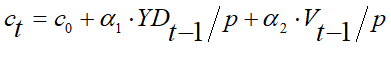
This is simply the wrong way to model time in an economic model, but it is the norm amongst economists of all paradigmatic persuasions. There is an alternative approach—which is the norm in genuine sciences—of modelling time using differential equations, and that’s what I will use in the remainder of this book.
Unfortunately, the practice of using discrete-time equations (otherwise known as “difference equations”: equations in terms of t, t-1, etc.) is so prevalent, and so accepted not just by Neoclassical economists, but by the staff who teach mathematical methods to young economists, that I have to spend some time dissing it first.
-
Friends Don’t Let Friends Use Difference Equations
Firstly, ask yourself, does your consumption today really depend on your income last year?
Of course not! Unless you are a billionaire, your expenditure today will be influenced by your income in the last week to month, not a year.
But that’s reasoning at the level of a single individual, and macroeconomic modelling, which is the focus of this book, is about aggregates. This brings in another level of distortion. The use of a difference equation for aggregate investment, for example implies that the investment decisions of all firms occur at the same frequency: that they are coordinated somehow. This is nonsense. Individual firms invest at very different frequencies to each other: a fast-food delivery service might invest on a monthly basis; a semiconductor producer might have a decade-long investment horizon.
The sum of many such asynchronous investment decisions ends up looking like a flow of investment decisions over time—which is the sort of thing that a differential equation portrays much more easily than a difference equation.
Thirdly, why do economic models use a one-year time-delay for everything? Fundamentally, because of laziness: it’s just easy to use a delay of 1 for everything.
There’s also a technical reason for this. Let’s say you took my criticism here seriously, but decided to still use difference equations, and to make your time-step a week rather than a year. Then you could have a difference equation for consumption with a time step of a week, which is reasonable, and one for investment with a time step of 52 weeks (a year), which is also reasonable. But then, to simulate your model you would need to provide 52 “initial conditions” for investment—if you had investment today depending on profits from 52 weeks ago, you would need to supply the model with 52 weekly values for profits (and investment) before it could be simulated.
Worse still, if you found by empirical research that the time delay in investment was actually 78 weeks, you would have to redesign your model to reflect that—and supply the additional 26 initial conditions as well.
This is where the laziness comes from: it’s so hard to do difference equations well, that economists do them badly instead, l and reduce everything to a one year time delay.
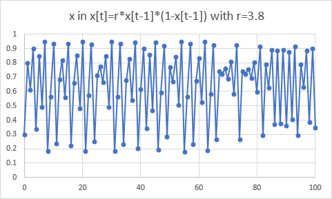
Fourthly, difference equations have some qualitative features that differ from those of differential equations, which can introduce spurious dynamics into a model. For example, I noted earlier that three dimensions are needed before a dynamic system can display complex behaviour—which used to be called “chaos”. But that’s only true of continuous-time equations. A one-dimensional difference equation can display chaotic behaviour, and one of the most famous such system is the logistic difference equation:
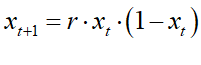
The pattern it generates is indeed fascinating—see Figure 11—and it has some real-world applications, notably in population dynamics for species with high reproduction rates.
Figure 11: Chaotic behaviour in the discrete-time logistic equation
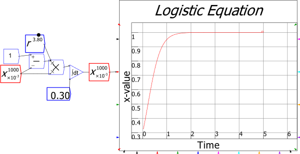
But if you’re trying to model a process in an economic model that has logistic characteristics, then using a discrete-time form, when the process is better described by the continuous form, will introduce spurious dynamics. Figure 12 shows how a continuous time logistic equation behaves. This might be more boring, but it will also be more realistic. A difference-equation model will generate more “interesting” dynamics, but simply because it uses the wrong modelling approach, not because the underlying economic system is truly chaotic (though as you will see, the macroeconomy can be chaotic—or rather complex).
Figure 12: Convergent behaviour in the continuous-time logistic equation
Some economists think that the discrete nature of economic data necessitates using discrete time models to reproduce it. The definitive riposte to this argument was given by the “father of system dynamics”, the engineer Jay Forrester, when he first encountered—and was seriously dismayed by—economic modelling in the 1950s. He observed that:
Time intervals of model solutions are often too widely spaced for the predictions being attempted. For example, a model solved annually to arrive at new annual values of economic variables would, if anything, be useful in predicting future trends over a five-year period but not year-to-year variations. As a rough rule-of-thumb, one would want solutions spaced closely enough to define a smooth curve through the fluctuations in which we are interested. {Forrester, 2003 #4915`, p. 334. Emphasis added}
In the concluding part of the paper, entitled “A future approach to model building”, Forrester reiterated that the belief that discrete data necessitated discrete modelling was simply wrong:
The incremental time intervals for which the variables of a model are solved step-by-step in time must be much shorter than often supposed… For models of the national economy as a whole it is unlikely that the time interval can be longer than one month and it is entirely possible that weekly intervals might be necessary.
This solution interval is unrelated to the interval at which national statistics and economic indicators are measured. The model should generate the instantaneous values of the variables which exist in the real system, whether or not these can be measured. The measurability of some of these variables is immaterial to the structure of the model and the incremental time steps through which it is advanced. The frequency of collection of statistics will only determine the frequency with which the model can be compared with reality, and in turn will affect the ease of getting the model structure and coefficients to converge toward their real counterparts.
The incremental time interval used for model solution will, on the other hand, be related to the lengths of the time constants which have been incorporated in the structure of the model. As a rough generalization, it will be necessary to have several solution intervals within the shortest time delay which is recognized in the model. Correspondingly, the model will need several solution intervals in a half-cycle of the highest frequency response which is to be generated at any point in the model. {Forrester, 2003 #4915`, p. 343. Emphasis added}
It might be thought that this would make mathematical modelling more complicated—wouldn’t the need for high frequency modelling force you to specify economic processes in intricate detail? In fact, the reverse is the case, because mathematicians have developed techniques for simulating dynamic systems that take care of the time intervals for you (the most famous being the Runge-Kutta algorithm), and these have adaptive mechanisms to improve simulation accuracy and speed as well. Rather than having to worry about the simulation time interval, you can forget about it, and well-established mathematical routines take care of it for you.
Another frequently made objection to continuous time methods is that economic decisions, such as investment, are based on lagged data, rather than current data, and therefore period analysis is needed to capture these lags. For example, Godley & Lavoie 2007 assume:
that governments react to lagged inflation rates, rather than to actual or expected inflation rates, on the realistic grounds that fiscal policy may have a reaction time somewhat longer than monetary policy. {Godley, 2007 #1240`, p. 92}
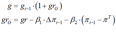
Therefore, they use the two equations shown in Equation to represent “real pure government expenditures” g, and the “growth rate of real pure government expenditures”, , where the rate of growth of government expenditure is a function of “the growth rate of potential output” gr, the change in the lagged inflation rate , and the deviation of the lagged inflation rate from the target inflation rate :
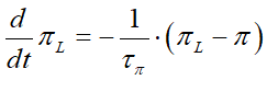
In fact, lags are easily represented in differential equations, using what is known as a “first-order time lag”, to relate the delayed perception of the rate of inflation to the actual, instantaneous rate of inflation . I’ll use rather than for the time-lagged inflation rate, since a time lag can be any length, not merely “one period”. The time-lagged inflation rate is defined by its rate of convergence to the actual inflation rate, which is given by the “time constant” (which, in an elaborate model, can be a variable if desired) which measures the length of time, in years, that it takes for the perceived rate of inflation to converge to the actual rate of inflation . If =0.5 this is a 6-month lag; if =1, a year, and so on. This rate of convergence is given by the differential equation shown in Equation :
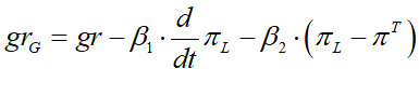
Similarly, the growth rate of government expenditure is expressed as a differential equation:
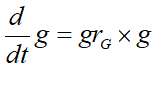
The variable growth rate can now defined as something like Equation , or it could be replaced with its own differential equation.
This approach is vastly superior to the discrete approach to time lags (which is more correctly called a time-delay, rather than a time-lag), for many reasons.
Time-lags are flexible. Your lag can be a fraction of a year, or multiple years, or even an irrational number if you wish: it doesn’t have to be 1,2, 3 “time periods”, as in conventional economic modeling. And of course, I’m being generous in saying that! As already noted, economic models use a time delay of “1 period” for almost everything. In Lavoie and Godley 2007, interest payments have a lag of -1 (equation 1); spending is negatively related to the interest rate with a lag of -1 (equation 2); taxes on wealth are lagged -1 (equation 7). This is typical. Factors which in the real world occur at vastly different frequencies—consumption, for example, has a much higher frequency than investment—are all corralled into the same arbitrary frequency.
Therefore, the time-delays (not time-lags) in discrete time economic models—which is to say, the vast majority of economic models—are spurious. They have nothing to do with the actual characteristics of time-dependent actions in the real economy. Time lags, on the other hand, can be derived from empirical data. They are also easy to edit: a time lag is a simple scalar, and if you find that you’re using the wrong value—say, data shows that the time lag in investment is actually 1.5 years when your model uses 3 years—then all you have to alter is that number. On the other hand, if discrete-time economic models did time delays properly, they would have different delays for consumption (short) versus investment (long). This simply isn’t done. If it were, and then empirical data indicated that the delay was different to what the model used, a wholesale re-writing of the model is necessary.
The final reason for economists using difference equations is simply habit. It’s what they’ve always done, therefore a century later, it’s what they still do: if there’s a difference equation approach at hand, that’s what they’ll use, even if differential equation methods are superior.
For that reason, I have not enabled difference equation logic at all in Minsky. Given how inappropriate difference-equation models are for modelling the economy, and yet how much they are used by economists, Minsky
deliberately does not support time-delays: “friends don’t let friends use periods”. We may need to introduce time-delays at some point, to enable the importing of models from other system dynamics programs, but if so, they will exist solely for that purpose.
With these issues covered, it’s time to turn from critique to construction.
-
A Simple Approach to Dynamics Using Ratios
Ordinary Differential Equations (ODEs) are hard, and “Partial Differential Equations” (PDEs) even more so. If you want to become truly fluent in dynamic modelling, then I recommend doing mathematics courses in calculus, differential equations, and linear algebra (which you need to work out the stability properties of dynamic systems).
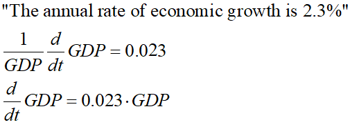
But it’s also possible to do a lot of dynamic modelling using something with which everyone is familiar: percentages (or rather, ratios). If you say, for example, that “the rate of growth of GDP is 2.3% per year”, you are stating a differential equation: you are saying that the rate of change of GDP equal 0.023 times the current value of GDP. The following are equivalent statements:
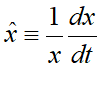
The ratio form is the most useful, since the logic of logarithms lets you convert division and multiplication of ratios into addition and subtraction. For example, if you have a variable x in your model, then mathematicians indicate its rate of growth by putting a “hat” over the variable:
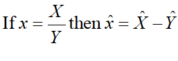
If x is the ratio of one variable X to another Y, then then the ratio of the rate of change can be converted into the rate of change ratio of X minus the rate of change ratio of Y:
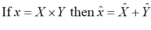
Similarly, the ratio of rate of change of the product of two ratios is the sum of their rates of change ratios:
This simple rule makes it surprisingly easy to build dynamic macroeconomic models using ratios. Macroeconomics abounds with definitions that are ratios: the employment rate, for example is the ratio of the number of people with a job to the population. It is therefore possible to start with a set of definitions and develop a dynamic model. I’ll illustrate this procedure in the next chapter.
-
A Simple Approach to Dynamics Using System Dynamics
System dynamics, which was invented by Jay Forrester in the 1950s, is simply a way to generate systems of ordinary differential equations. So long as the flowchart forms a causal loop, it generates a set of differential equations which can be of daunting complexity. But if you can read the flowchart, you can understand the model.
Building an insightful system dynamics model isn’t easy, but it is far easier than the laborious methods that Neoclassical economists use to purport to derive macroeconomic models from microeconomic: when Blanchard noted that the fool’s errand of deriving a macroeconomic model from microeconomic concepts implied “a long slog from the competitive model to a reasonably plausible description of the economy” {Blanchard, 2016 #5194`, p. 3}, he wasn’t joking. I remember discussing modelling some detail of the monetary system with Michael Kumhof of the Bank of England—who is the only Neoclassical economist who understands that banks create money {Kumhof, 2015 #5120. Michael remarked it would take of the order of months to add it to his DSGE model. I replied that it would take me of the order of minutes to do the same thing in Minsky. I’ll illustrate that point in the next few Chapters.