Abstract
Modern Monetary Theory (MMT) is a non-mainstream economic theory that contradicts conventional economic analysis of government debt and deficits. We use the system dynamics program Minsky to develop a mathematical model of MMT. This model shows that the core tenets of MMT are correct, and Neoclassical arguments about government debt and deficits are wrong.
Introduction
A common criticism of MMT by Neoclassical economists is that it lacks a mathematical framework:
MMT theorists have never subjected their theory to formal treatment by mathematical modeling (Bossone 2021, p. 162).
MMT lacks theoretical analysis based on mathematical models compared to mainstream economics, which is based on a neoclassical framework. (Tanaka 2021, p. 2)
These critics then proceed to examine MMT using the tools of Neoclassical economic theory:
the choice of using ISLM analysis for the purpose of this article is not driven by which model should best describe the economy in general, but rather by which model can best mirror the economic relations underpinning MMT, in the absence of a formal representation by its proponents, while subjecting them to consistency checks. (Bossone 2021, p. 163. Emphasis added)
In this paper, we try to argue positively for the idea of the effect of fiscal policy, which is the backbone of functional finance theory and MMT’s argument, using a simple mathematical model, while maintaining the basics of the neoclassical microeconomic framework, such as utility maximization of consumers by utility function and budget constraint [sic.], profit maximization of firms in monopolistic competition, and equilibrium of supply and demand of goods. (Tanaka 2021, p. 2. Emphasis added)
A common retort by MMT economists is that Neoclassical models of money are simply wrong. Kelton observes that:
MMT rejects the loanable funds story, which is rooted in the idea that borrowing is limited by access to scarce financial resources. As MMT economist Scott Fullwiler put it, the conventional “analysis is simply inconsistent with how the modern financial system actually works.” (Kelton 2020, p. 113)
If the conflict between these two paradigms is to be resolved, we need a mathematical framework which is consistent with how the modern financial system actually works. The Open-Source system dynamics program Minsky provides that framework.
Minsky, the software
Minsky is named in honour of the great Post-Keynesian economist Hyman Minsky (Minsky 1982), who developed the “Financial Instability Hypothesis” (Minsky 1977) as a realistic alternative to the Neoclassical “Efficient Markets Hypothesis”, which underlies the “Capital Asset Pricing Model” (Fama and French 2004; Sharpe 1964). Minsky supports the standard system dynamics tools of flowchart modelling,
and in addition
provides Godley Tables—named after another great Post-Keynesian, Wynne Godley (Godley 1999)—which enable easy modelling of financial stock and flows.
A Godley Table records financial transactions following the principles of double-entry bookkeeping (Gleeson-White 2011), that:
- All financial claims are classified as either Assets or Liabilities;
- One entity’s financial Asset is another entity’s financial Liability; and
- All transactions are recorded twice, subject to the fundamental rule of accounting that Assets (A) minus Liabilities (L) equals Equity (E).
The entries in a Godley Table generate a set of differential equations describing the model of the financial system. So long as every transaction is properly recorded, then the model is structurally correct.
Figure 1 shows a blank Godley Table.
Figure 1: A blank Godley Table (as seen in the Edit window)
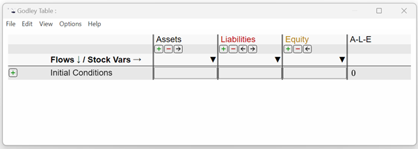
Stocks (financial assets and liabilities) are defined on the row beginning “Flows¯/Stock Vars®” in Figure 1, and are added, deleted and moved using the +,- and ¬® buttons. Flows (financial transactions) are defined on the rows of the Table, with two entries required per row. These entries must obey the rule that , which is checked by the final column in the table. Minsky uses the rule that one entity’s asset is another’s liability to enable an integrated model of the financial system to be developed. The wedge symbol q accesses a drop-down menu showing Assets that have not yet been recorded as Liabilities for another entity, and vice versa.
A quick primer on Minsky
Figure 2 shows a simple economic model, in which bank lending creates both Loans and Deposits. Borrowers then pay interest, and the banks purchase goods and services from the non-bank private sector.
Figure 2: A simple model of bank-originated money and debt
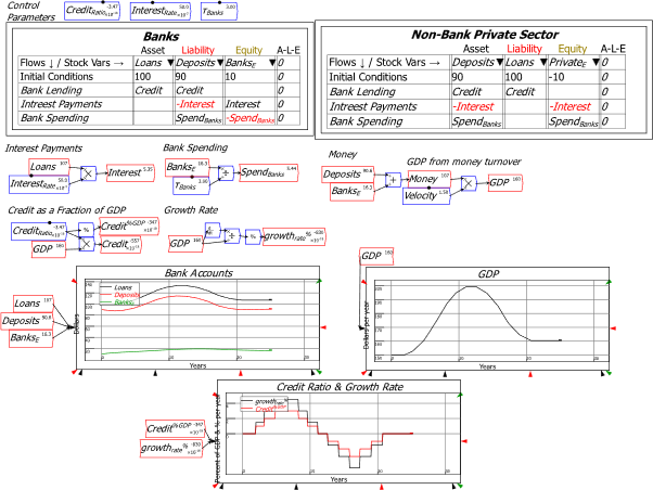
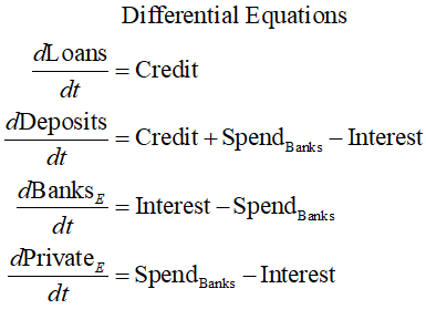
The Godley Tables generate the differential equations of the model, since the symbolic sum of a column is the rate of change of the relevant stock:
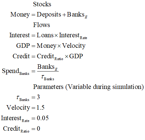
The flows are defined on the design canvas using mathematical operators. Variables and parameters can be copied and used in multiple locations on the canvas if desired. Parameter values can be altered during a simulation, using either arrow keys or the “dot” slider on top of the parameter.
Minsky generates the equations for the model, which can be exported in LaTeX format for documentation purposes—see Equation (1) and (2).
This model could easily be developed in any system dynamics program using flowchart logic, but there is an enormous advantage in using Godley Tables instead. The entire financial system operates on the principles of double-entry bookkeeping, which has the same status In the analysis of monetary systems as the Laws of Thermodynamics have in the analysis of energy. We therefore paraphrase Sir Arthur Eddington’s marvellous put-down of models in physics that violate the Second Law of Thermodynamics (Eddington 1928, p. 37):
The rules of double-entry bookkeeping hold the supreme position among the laws of Money. If your theory is found to be against the rules of double-entry bookkeeping, we can give you no hope; there is nothing for it but to collapse in deepest humiliation.
Minsky‘s Godley Tables ensure that these rules are obeyed, and it therefore acts not only as an enabler of accurate financial modelling, but also as a prohibition: actions which might be possible to model in standard flowchart notation can violate double-entry bookkeeping, and are therefore wrong.
A clear example here is the model of “Fractional Reserve Banking”, which gives rise to the “Money Multiplier” theory of money creation, and which is taught by all conventional economic textbooks. This is an extract from the popular textbook Principles of Macroeconomics by Mankiw:
Deposits that banks have received but have not loaned out are called reserves… After the bank opens and people deposit their currency, the money supply is the $100 of demand deposits… Let’s suppose that First National has a reserve ratio of … 10 percent … it keeps 10 percent of its deposits in reserve and loans out the rest… It turns out that even though this process of money creation can continue forever, it does not create an infinite amount of money. If you laboriously add the infinite sequence of numbers in the preceding example, you find the $100 of reserves generates $1,000 of money. (Mankiw 2016, pp. 332-334)
This model is also clearly believed by economic policymakers. This is how then Federal Reserve Chairman Ben Bernanke explained why Quantitative Easing was being undertaken in the aftermath to the Global Financial Crisis:
Large increases in bank reserves brought about through central bank loans or purchases of securities are a characteristic feature of the unconventional policy approach known as quantitative easing. The idea behind quantitative easing is to provide banks with substantial excess liquidity in the hope that they will choose to use some part of that liquidity to make loans or buy other assets. (Bernanke 2009, p. 5. Emphasis added)
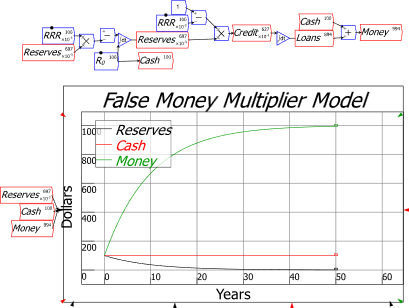
This process of “lending out Reserves” is easily modelled using the flowchart method: see Figure 3.
Figure 3: The “Money Multiplier” portrayed in a conventional system dynamics format
However, when this model is laid out using a Godley Table, there is an obvious problem: directly “lending from Reserves” violates double-entry bookkeeping: see Figure 4.
Figure 4: Lending directly from Reserves violates the fundamental rules of accounting
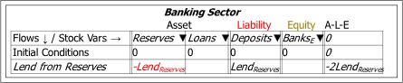
Figure 4 is doubly wrong because it also doesn’t create any loans. The only way to show Loans being created is to have Reserves fall and Loans rise by the same amount, as in Figure 5.
Figure 5: No violation of accounting, but how do borrowers get the money?
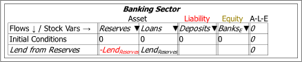
This now accords with the rules of accounting, but at this stage there is an additional liability for borrowers (increased Loans) but no additional assets (increased money). To show borrowers getting money from the loans, we have to include the Private Sector’s Godley Table, and show that some other Private Sector asset rises to compensate for this increase in the Private Sector’s liabilities. This asset is Cash: the borrowers’ cash holdings rise by the amount of the loans, and the borrowers then re-deposit this cash at the banks—see Figure 6.
Figure 6: The Money Multiplier only works if the entire monetary system operates with cash
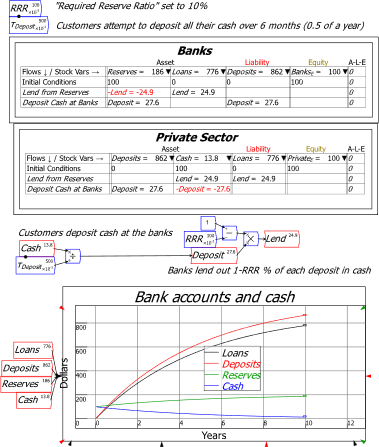
The simple model now works as a way to create money, but only under two absurd conditions: not only must all loans be in cash, the entire monetary system—including Reserves—must be cash-based. You can get rid of needing Reserves to be cash-based by a much more complicated model, but you cannot escape the requirement that loans themselves must be in cash.
This is fallacious as a description of modern banking. While it may have been approximately the case in the 19th century, it is ridiculous today, when the vast majority of loans are electronic.
Mainstream economic models of money—both the “Money Multiplier” and “Loanable Funds”—face humiliation when expressed in terms of double-entry bookkeeping. The core tenets of MMT, on the other hand, are derived from the principles of double-entry bookkeeping.
MMT
The Government Deficit is the Private Surplus
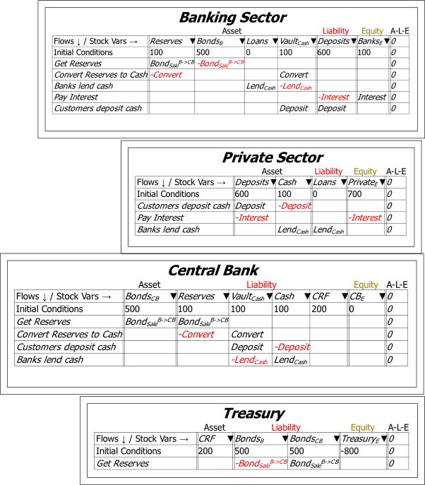
Figure 7 shows the essential government operations of spending and taxation as seen from the point of view of the Banking Sector.
Figure 7: Government spending and taxation shown on the Banking Sector’s Godley Table
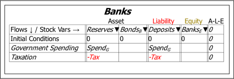
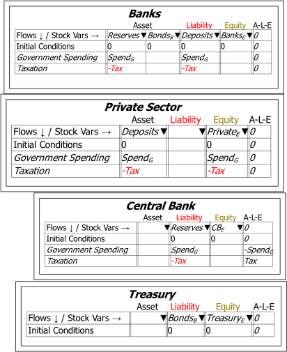
As with the private money creation dynamics outlined in Figure 2, these entries cascade through the financial accounts of the other sectors—shown via Godley Tables in Minsky. Reserves are a Liability of the Central Bank, while Bonds are a Liability of the Treasury. Figure 8 shows the consequences of laying out the transactions in Figure 7 for the other sectors, and this shows that the model is incomplete: there is as yet no account against which to record the second double-entry for both spending and taxation on the Central Bank’s table.
Figure 8: The basic but incomplete view of government spending and taxation
This indicates that there is another account which must be added to the model: the Treasury’s account at the Central Bank. This is commonly known as the Consolidated Revenue Fund (CRF), and we call it TreasuryCRF here. Figure 9 shows this completed fundamental model.
Figure 9: The basic complete view of government spending and taxation
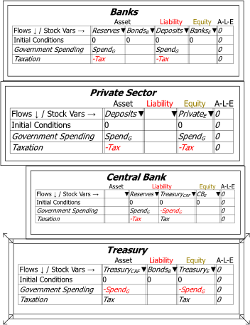
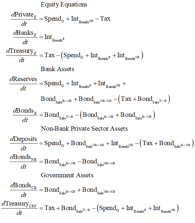
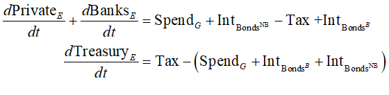
Figure 9, and the equations of this model in Equation , confirm the core MMT insight that the government deficit IS the private sector surplus. If government spending exceeds taxation, then the private sector’s net financial worth—its equity—rises by , which is precisely the sum by which the government sector’s net financial worth falls. This is obvious in the non-zero differential equations which Minsky generates from the tables in Figure 9:
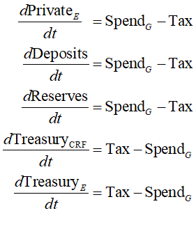
The MMT ab-initio argument first made by Warren Mosler (Mosler 2010), that the government must spend before it can tax, is also confirmed by these equations. For fiat money to exist, the government must first spend it into existence.
This explains the fundamental nature of fiat money. Fiat money is created by a government issuing net financial liabilities upon itself, which in turn creates net financial assets for the non-government sector.
If the government does not spend more than it takes back in taxation, then it does not create fiat money—and a surplus actually destroys fiat money. Mainstream economists who object to the government running a deficit are in fact objecting to the creation of fiat money.
Fiat money gives the non-government sector a means to undertake monetary transactions by exchanging the government’s liabilities—fiat money—with each other. Without fiat money, the only liabilities that can be exchanged are those created by the banking sector: credit money. Fiat money creation also increases the net financial worth of the non-government sector, whereas credit-based money does not.
Finally, both credit and fiat money creation work by increasing the Assets of the Banking Sector simultaneously with increasing the Liabilities. Credit money creation increases Loans, which are an income earning asset for the Banking Sector. Fiat money creation increases Reserves, which—prior to the Global Financial Crisis (GFC)—were not an income-earning asset for the Banking Sector.
A Conservation Law
Minsky reveals a fundamental but thus far overlooked aspect of a monetary economy: the conservation law that the sum of all financial equities is zero. Since every entity’s financial asset is another entity’s financial liability, in the aggregate, the net financial equity of every sector identically equals the negative of the net financial equity of all other sectors. This mathematical truism provides a reason to support fiat money—and hence government deficits—that even Austrian economists might be able to comprehend: without government deficits, the non-bank private sector is necessarily in negative financial equity.
A bank must have positive net worth: its short-term assets must exceed its short-term liabilities, otherwise it is bankrupt. Therefore, in the absence of a government sector, the non-bank private sector must be in negative equity: its financial liabilities must exceed its financial assets. However, with a government sector that is in sufficient negative equity, it is possible for both the private banking sector and the non-bank private sector to be in positive financial equity.
There has never been an economy without a government, of course, but America in the 19th century and up until WWII provides an example of an economy with a very small government sector (relative to GDP) compared to the post-WWII economy. On several occasions, the government succeeded—for want of a better word—in reducing its debt to zero. This achievement—driven by the same misplaced abhorrence of government negative equity that lies behind today’s politicians desire to reduce government debt—necessarily drove the private non-bank sectors into negative equity. This may well be a factor in the many financial crises that afflicted the US economy up until the start of WWII.
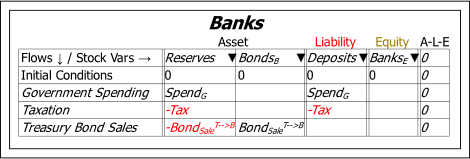
Treasury Bond Sales
Technically speaking, Figure 9 and Equations (2) and describe the only essential operations in fiat money creation. However, governments have imposed additional requirements upon the operations of the Treasury and Central Banks via laws that require the CRF to not be in overdraft, and which prevent the Central Bank from buying bonds directly from the Treasury. We therefore have to introduce Treasury Bond sales in Primary Auctions, and Central Bank purchases of bonds on the Secondary Market.
Treasury bond sales to the banking sector are shown as the flow BondSaleTàB in Figure 10. These are purchased by the banking sector using its Reserves—and these Reserves are created in the first instance by the government deficit.
This confirms the key MMT insight that the funds banks use to buy government bonds are created by the deficit itself. The purchase of the bonds neither creates money, nor takes money from the private sector, since both transactions occur only on the Asset side of the Banking Sector’s ledger. Treasury Bond sales to the Banking Sector are an asset swap for the banks: they do not constitute borrowing (though they do initiate interest payments, which we consider next). Exchanging Reserve funds for Bonds enables banks to part with a non-tradeable asset (and until the GFC, non-income-earning asset) which was created by the Treasury, for a tradeable, income-earning asset which was also created by the Treasury.
Figure 10: Sales of Treasury Bonds to the Banking Sector
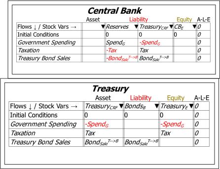
The main practical impact of this transaction is on the Treasury’s account at the Central Bank. If the government habitually runs a deficit, then its account at the Central Bank will have more outflows than inflows, and will necessarily turn negative. Almost all governments have passed laws requiring their Treasuries not to be in overdraft to the Central Bank, and this is what Bond sales achieve: if Bond sales are equal to the deficit, then the Treasury’s Consolidated Revenue Fund (CRF) at the Central Bank can remain non-negative—see Figure 11.
Figure 11: The government sector view of Treasury Bond sales
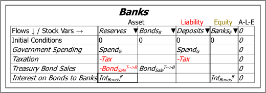
Interest on Treasury Bonds
Introducing bond sales made no difference to government money creation. Interest on bonds, on the other hand, does. Figure 12 shows that interest on bonds owned by Banks adds to the net worth of the Banking Sector.
Figure 12: Interest on Bonds from the Banking Sector’s Perspective
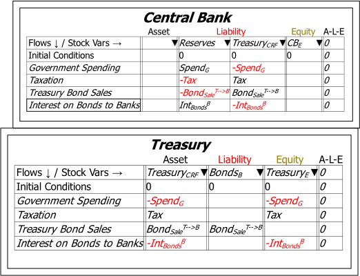
This necessarily increases the negative net financial worth of the government sector. The rate of change of the Treasury’s equity now equals —see Figure 13. Maintaining a non-zero balance in the Treasury’s CRF requires the Treasury to issue bonds equivalent to the deficit plus interest on outstanding bonds held by the non-government sector.
Figure 13: Interest on Bonds from the Government’s Perspective
Central Bank Open Market Operations
A notable feature of the model thus far is that the Central Bank has no assets. This is addressed by considering Central Bank Open Market Operations (OMO). Though these are undertaken primarily to keep the interest rate on bonds within the Central Bank’s target range, the effect of net Bond purchases by the Central Bank is to create positive assets it. If, hypothetically, these net purchases equal the interest paid on bonds owned by the Government sector, then the potential for the exponential growth of government “debt” (in reality, of Treasury bonds owned by the non-Government sector), which has led to some internet chatter in recent months, will not be realised, since around the globe, Treasuries either do not pay interest on bonds owned by other sectors of the government, or Central Banks remit their earnings to the Treasury.
Figure 14: Open Market Operations by the Central Bank
Bank Sales of Bonds to Non-Banks
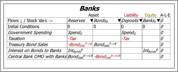
The final detail needed to portray the basic operations of fiat money creation is the sale of bonds by banks to the non-bank private sector—and primarily to Non-Bank Financial Institutions (NBFIs). This is one of the only two bond operations which change the amount of money in the economy—the other being Open Market Operations (including “Quantitative Easing” and “Quantitative Tightening”) with NBFIs. Bonds sales by Banks to NBFIs are executed by debiting the deposit accounts of NBFIs at the Banks, which reduces the money supply.
These operations complete the basic double-entry-based view of the operations involved in fiat money creation. The full structure is shown in Figure 15.
Figure 15: The complete structural model of fiat money operations
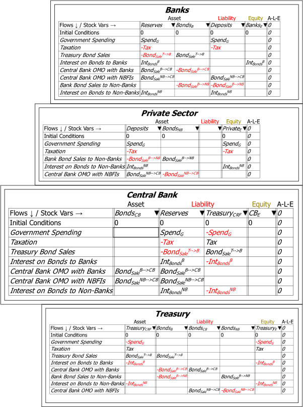
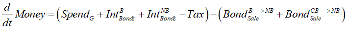
The non-zero differential equations of this process are shown in Equation :
A Summing Up
The main characteristics of this systemic description of government finances, derived directly from double-entry bookkeeping, are:
- Government spending in excess of taxation is financed by the government going into negative financial equity to the same magnitude, which creates equivalent positive financial equity for the non-government sectors. The condition under which the government creates positive financial equity for the non-government sector is:
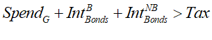
- In this simple model, the money supply is the sum of Deposits and the banking sector’s short-term equity BanksE. The operation in Equation creates money for the non-government sectors, so long as this positive equity is greater than bond sales to non-banks by the private banks and Central Bank:
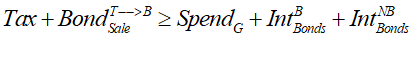
- Bond sales by the Treasury are undertaken to maintain a non-negative balance for the Treasury’s Consolidated Revenue Fund at the Central Bank. This condition will hold so long as:
- The funds used by the banking sector to buy government bonds are created by the government Deficit—the excess of government spending and interest payments over taxation—which increases the Banking Sector’s Reserves; the money used by the non-bank private sector to buy bonds is created the same way, since the Deficit also creates Deposits; and
- Interest on government bonds is a fiat-money-financed source of income for the private sector.
These deductions are all consistent with the basic tenets of MMT, as set out in The Deficit Myth (Kelton 2020). In contrast, the attitudes of Neoclassical economics towards budget deficits are inconsistent with double-entry bookkeeping.
The Neoclassical Approach to Budget Deficits
Mankiw’s textbook Principles of Macroeconomics (Mankiw 2016) is typical of the Neoclassical treatment of government deficits. Mankiw situates his analysis within the model of Loanable Funds:
To keep things simple, we assume that the economy has only one financial market, called the market for loanable funds. All savers go to this market to deposit their saving, and all borrowers go to this market to take out their loans. Thus, the term loanable funds refers to all income that people have chosen to save and lend out, rather than use for their own consumption, and to the amount that investors have chosen to borrow to fund new investment project (Mankiw 2016, p. 268)
Supply and demand analysis, and not double-entry bookkeeping, is thus the foundation of the Neoclassical critique of MMT. The correct domain of supply and demand analysis is the production and consumption of goods and services, and even there it has enormous problems (Keen 2024; Keen 2021, 2011). Here, supply and demand analysis in the form of Loanable Funds ignores double-entry bookkeeping, and does not explain the creation of money: instead, it takes the money supply as given, and discusses its allocation, in that any money that is not spent on consumption is assumed to be the source of loanable funds:
The supply of loanable funds comes from people who have some extra income they want to save and lend out… saving is the source of the supply of loanable funds. (Mankiw 2016, p. 268)
One of several fallacies in this analysis is the lumping together of public and private savings, as if they are independent activities:
When the government runs a budget deficit, public saving is negative, and this reduces national saving. In other words, when the government borrows to finance its budget deficit, it reduces the supply of loanable funds available to finance investment by households and firms. (Mankiw 2016, p. 273)
This is easily shown to be false using the Equity Equations in Equation (4). Savings can be defined as the change in equity of an entity, and private saving is the sum of the change in equity of the non-government private sectors (bank and non-banks). This is identically equal to the negative of the change in equity for the government sectors (Central Bank and Treasury). The correct equation is:
Mankiw’s first sentence is thus 100% wrong. The correct statement of the relation between the budget deficit and private savings is:
When the government runs a budget deficit, public saving is negative, and this creates private savings. In other words, when the government runs a deficit, it increases the supply of bank deposits available to finance consumption and investment by households and firms.
Mankiw also asserts that a government deficit decreases the supply of funds available for private investment:
Thus, the most basic lesson about budget deficits follows directly from their effects on the supply and demand for loanable funds … the government reduces national saving by running a budget deficit … The model as presented here takes this term [Loanable Funds] to mean the flow of resources available to fund private investment; thus, a government budget deficit reduces the supply of loanable funds… a budget deficit increases the interest rate, thereby crowding out private borrowers who are relying
on financial markets to fund private investment projects. (Mankiw 2016, p. 274. Emphasis added)
These deductions are the exact opposite of the real impact of government deficits. The deficit increases the money supply, and therefore the money available to the private sector for both investment and consumption expenditures. This is likely to reduce the demand for credit-based money, which if anything will reduce commercial interest rates, and/or increase the level of investment.
Disentangling Cause and Effect with Minsky
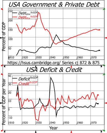
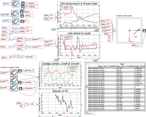
Advocates of austerity often point to the prosperity of years in which America ran surpluses and reduced government debt—specifically the Coolidge and Clinton Presidencies. Predictably—given the mainstream attitude that lending is a “pure redistribution” which should have “no significant macroeconomic effects” (Bernanke 2000, p. 24)—they ignore what happened to private debt at the same time. As federal debt fell from 27% of GDP in 1920 to 16% in 1929, private debt rose from 121% to 156%: see Figure 16.
Figure 16: Debt, Deficits and Credit from 1916-1976
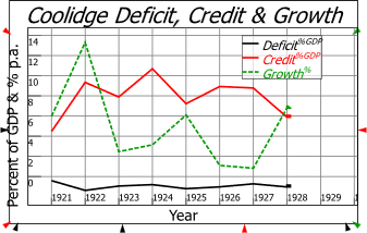
Thus, as the Coolidge administration ran a surplus of 1% of GDP, private sector credit grew at an average of 8% of GDP per year—see Figure 17.
Figure 17: The Deficit, Credit and Growth 1921-28
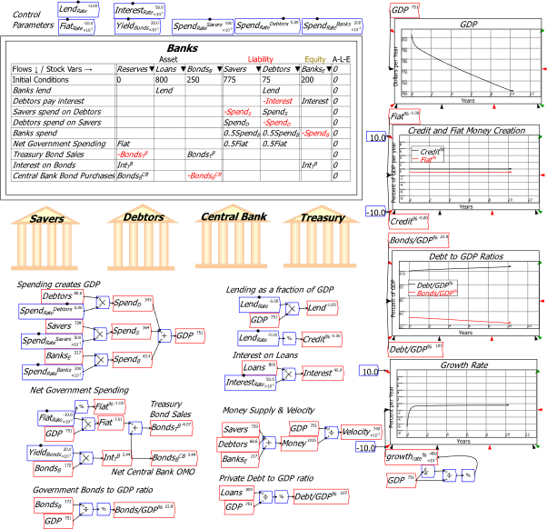
Minsky enables us to untangle these two factors to see what really caused the growth of the 1920s, by creating a model with both credit and fiat money creation—see Figure 18:
Figure 18: A simple mixed fiat and credit model in Minsky
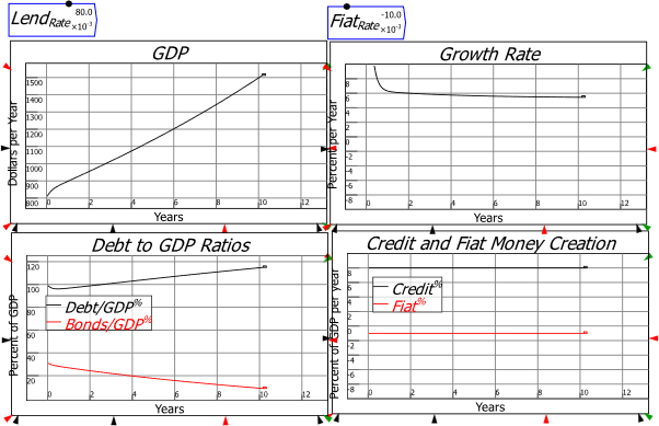
Reproducing the average rates of credit growth and fiat money contraction in the 1920s caused by Coolidge’s surpluses reproduces much the same economic outcomes: a high rate of economic growth, a falling government debt ratio, and a rising private debt ratio—see Figure 19.
Figure 19: A 1% of GDP surplus and 8% of GDP credit growth reproduces the 1920s data
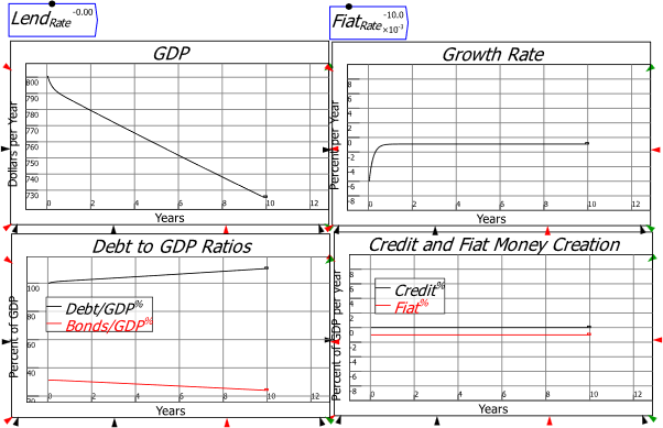
However, the counterfactual of a 1% of GDP surplus with no credit growth produces an entirely different outcome: the one that MMT predicts of a declining GDP—see Figure 20.
Figure 20: Coolidge’s surplus on its own reduces economic growth
Other Aspects of Minsky for system dynamics experts
This paper focuses upon Minsky‘s capabilities in the topic area which inspired its creation, but there are also aspects of Minsky which should be of interest to practitioners of system dynamics in general.
Firstly, Minsky is one of the few system dynamics programs which are both Open Source and free. You can download it from https://sourceforge.net/projects/minsky/.
Secondly, Minsky‘s design philosophy emphasizes transparency: relationships between stocks and flows are explicitly modelled on the canvas, rather than inside text boxes as in the majority of system dynamics programs. Minsky passes values “by name” as well as “by wire”, so the spaghetti diagrams of conventional programs are replaced by much smaller “spiders’ webs” which define parts of a model. This makes it easier to explain a model to a non-specialist.
Thirdly, since it is programmed by a high-performance-computing expert with a PhD in physics, Dr Russell Standish, Minsky is much more “math-centric” than conventional system dynamics programs. It supports tensor mathematics, produces the equations of its models in LaTeX, and provides symbolic rather than simply numerical differentiation.
Minsky also lacks some tools that professional system dynamics modelers rely upon—such as methods to identify loop dominance. We hope to add such features over time, and financial support via Minsky‘s Patreon page https://www.patreon.com/hpcoder/ will help enable this.
However, we realise that voluntary support alone is unlikely to provide sufficient development funds, while system dynamics is still too “esoteric” a field for most system dynamics programs to be commercially viable.
We have therefore developed a commercial extension of Minsky called Ravel, which is targeted at the spreadsheet, Pivot Table, and “Business Intelligence” marketplace. Ravel uses a novel and patented tool for manipulating multidimensional data visually—see Figure 21. We hope that sales revenue from Ravel will enable us to continue developing Minsky for the system dynamics community. Ravel should be available from mid-2024, and will initially be marketed via Patreon.
Figure 21: Ravel uses Minsky’s interface and the Ravel© object to analyse multidimensional data
Why are mainstream models of money so bad?
Mainstream models of money are fallacious, and rely upon obviously false assumptions—that all loans are in cash (the Money Multiplier) or that bank deposits aren’t demand deposits, and that loans aren’t bank assets (Loanable Funds).
It is therefore not MMT that fails the test of mathematical analysis, but mainstream macroeconomics, with its obsession with equilibrium, and its wilful ignorance of the monetary system. But there is little chance of using system dynamics to persuade mainstream economics to abandon its fallacious models of money and adopt realistic ones, because that would result in the rapid unwinding of the entire Neoclassical paradigm.
The core reason that Neoclassical models of the monetary system are so infantile is that their core paradigm ignores money, and treats capitalism as a barter system. Their models of money are therefore not attempts to describe the monetary system, but attempts to justify ignoring the monetary system in macroeconomic modelling.
Their treatment of groundbreaking papers by Central Banks on money creation is indicative here. In 2014, the Bank of England published “Money creation in the modern economy” (McLeay, Radia, and Thomas 2014), which bluntly rejected mainstream models of money creation and endorsed the non-mainstream “Post-Keynesian” models:
Money creation in practice differs from some popular misconceptions — banks do not act simply as intermediaries, lending out deposits that savers place with them, and nor do they ‘multiply up’ central bank money to create new loans and deposits. (McLeay, Radia, and Thomas 2014, p. 14)
This paper—and a similar one from the Bundesbank (Deutsche Bundesbank 2017)—was largely ignored by mainstream economists, while one of the few papers that engaged with it argued that “loanable funds” was preferable to “the money-creation approach” via a bizarre version of “Occam’s Razor”:
We establish a benchmark result for the relationship between the loanable-funds and the money-creation approach to banking. In particular, we show that both processes yield the same allocations when there is no uncertainty. In such cases, using the much simpler loanable-funds approach as a shortcut does not imply any loss of generality. (Faure and Gersbach 2017, p. 107. Emphasis added)
Only Neoclassical economists could combine the words “when there is no uncertainty” with “does not imply any loss of generality” in the one paragraph.
Conclusion
Forrester’s motivation for developing system dynamics can arguably be traced back to his justified incredulity at the state of mathematical modelling in economics in the 1950s. In the note “Dynamic models of economic systems and industrial organizations: Note to the Faculty research seminar. From Jay W. Forrester. November 5, 1956” (Forrester 2003), he made the following observations:
One of the striking shortcomings of most economic models is their failure to reflect adequately the structural form of the regenerative loops that make up our economic system…
Present models neglect to interrelate adequately the flows of goods, money, information, and labor…
Linear equations have usually been used to describe a system whose essential characteristic, I believe, arise from its non-linearities…
Models, suitable only for long-range prediction, are often used with short-term influences and fluctuations omitted. This is justifiable only if the system is sufficiently linear to permit superposition, an assumption which has not been justified or defended and which is probable untrue…
Time intervals of model solutions are often too widely spaced for the predictions being attempted…
Very often the model and its results are judged by the logic with which the model is developed out of its founding assumptions, whereas the failures probably lie in those assumptions. (Forrester 2003, pp. 332-336)
These criticisms remain valid today, while the economics discipline greeted the first large-scale system dynamics model (Forrester 1971) with both hostility and ignorance (Forrester, Gilbert, and Nathaniel 1974; Nordhaus 1973). The dominant paradigm, Neoclassical economics, remains implacably opposed to methods that do not enforce equilibrium as an outcome of a model (Lazear 2000; Blanchard 2018).
The only hope for getting economists to use system dynamics in place of its current reliance upon either algebraic or discrete-time modelling tools is to partner with economists who are dedicated to realism rather than ideology. These economists self-describe themselves as either Post-Keynesian or Modern Monetary Theorists, or both. However, these groups are often unfamiliar with the methods of system dynamics, and use technologies—such as discrete-time modelling (Lavoie and Zezza 2020)—out of the habits of their training, rather than knowledge of the most appropriate tools.
Minsky is the only tool which enables system dynamic modelling in economics, while enforcing a correct analysis of financial flows. We encourage the system dynamics community to become familiar with Minsky, and to support the subcultures within economics that wish to embrace the realism of dynamics, rather than the fantasy of equilibrium.
Appendix
Figure 22: The Money Multiplier Model with electronic reserves
References
Bernanke, Ben. 2009. “The Federal Reserve’s Balance Sheet: An Update.” In Federal Reserve Board Conference on Key Developments in Monetary Policy. Washington, DC: Board of Governors of the Federal Reserve System.
Bernanke, Ben S. 2000. Essays on the Great Depression (Princeton University Press: Princeton).
Blanchard, Olivier. 2018. ‘On the future of macroeconomic models’, Oxford Review of Economic Policy, 34: 43-54.
Bossone, Biagio. 2021. ‘Why MMT can’t work’, International Journal of Economic Policy Studies, 15: 157-81.
Carter, Susan B. 2006. Historical statistics of the United States : earliest times to the present / editors in chief, Susan B. Carter … [et al.] (Cambridge University Press: New York).
Deutsche Bundesbank. 2017. ‘The role of banks, non- banks and the central bank in the money creation process’, Deutsche Bundesbank Monthly Report, April 2017: 13-33.
Eddington, Arthur Stanley. 1928. The Nature Of The Physical World (Cambridge University Press: Cambridge).
Fama, Eugene F., and Kenneth R. French. 2004. ‘The Capital Asset Pricing Model: Theory and Evidence’, The Journal of Economic Perspectives, 18: 25-46.
Faure, Salomon A., and Hans Gersbach. 2017. “Loanable funds vs money creation in banking: A benchmark result.” In CFS Working Paper Series. Frankfurt: Center for Financial Studies (CFS), Goethe University.
Forrester, Jay W. 1971. World Dynamics (Wright-Allen Press: Cambridge, MA).
———. 2003. ‘Dynamic models of economic systems and industrial organizations: Note to the Faculty research seminar. From Jay W. Forrester. November 5, 1956’, System Dynamics Review, 19: 329-45.
Forrester, Jay W., W. Low Gilbert, and J. Mass Nathaniel. 1974. ‘The Debate on “World Dynamics”: A Response to Nordhaus’, Policy Sciences, 5: 169-90.
Gleeson-White, Jane. 2011. Double Entry (Allen and Unwin: Sydney).
Godley, Wynne. 1999. ‘Money and Credit in a Keynesian Model of Income Determination’, Cambridge Journal of Economics, 23: 393-411.
Keen, S. 2024. “Rebuilding Economics from the Top Down.” In. Budapest: Budapest Centre for Long-Term Sustainability & Pallas Athene Publishing House.
Keen, Steve. 2011. Debunking economics: The naked emperor dethroned? (Zed Books: London).
———. 2021. The New Economics: A Manifesto (Polity Press: Cambridge, UK).
Kelton, Stephanie. 2020. The Deficit Myth: Modern Monetary Theory and the Birth of the People’s Economy (PublicAffairs: New York).
Lavoie, Marc, and Gennaro Zezza. 2020. ‘A Simple Stock-Flow Consistent Model with Short-Term and Long-Term Debt: A Comment on Claudio Sardoni’, Review of Political Economy, 32: 459-73.
Lazear, Edward P. 2000. ‘Economic Imperialism’, Quarterly Journal of Economics, 115: 99-146.
Mankiw, N. Gregory. 2016. Principles of Macroeconomics, 9th edition (Macmillan: New York).
McLeay, Michael, Amar Radia, and Ryland Thomas. 2014. ‘Money creation in the modern economy’, Bank of England Quarterly Bulletin, 2014 Q1: 14-27.
Minsky, Hyman P. 1977. ‘The Financial Instability Hypothesis: An Interpretation of Keynes and an Alternative to ‘Standard’ Theory’, Nebraska Journal of Economics and Business, 16: 5-16.
———. 1982. Can “it” happen again? : essays on instability and finance (M.E. Sharpe: Armonk, N.Y.).
Mosler, Warren. 2010. “The Seven Deadly Innocent Frauds.” In.: Valance Co., Inc.
Nordhaus, William D. 1973. ‘World Dynamics: Measurement Without Data’, The Economic Journal, 83: 1156-83.
Sharpe, William F. 1964. ‘Capital Asset Prices: A Theory of Market Equilibrium under Conditions of Risk’, The Journal of Finance, 19: 425-42.
Tanaka, Yasuhito. 2021. ‘An Elementary Mathematical Model for MMT (Modern Monetary Theory)’, Research in Applied Economics.