In contrast to its attitude to private debt, which it ignores, mainstream economics obsesses about government debt. But this volte-face doesn’t besmirch its record of being 100% wrong.
Government debt, mainstream economics tells us, is a scourge to be minimized, if it can’t be entirely avoided. These quotes are from Mankiw’s influential macroeconomics textbook (Mankiw 2016), with indicative passages highlighted:
When a government spends more than it collects in taxes, it has a budget deficit, which it finances by borrowing from the private sector or from foreign governments. The accumulation of past borrowing is the government debt… (555)
The government debt expressed as a percentage of GDP roughly doubled from 25 percent in 1980 to 47 percent in 1995. The United States had never before experienced such a large increase in government debt during a period of peace and prosperity. Many economists have criticized this increase in government debt as imposing an unjustifiable burden on future generations… (557)
These trends led to a significant event in August 2011: Standard & Poor‘s, a major private agency that evaluates the safety of bonds, reduced its credit rating on U.S. government debt to one notch below the top AAA grade. For many years, U.S. government debt was considered the safest around. That is, buyers of these bonds could be completely confident that they would be repaid in full when the bond matured. Standard & Poor’s, however, was sufficiently concerned about recent fiscal policy that it raised the possibility that the U.S. government might someday default. (559)
Increases in government debt are a concern because they place a burden on future generations of taxpayers and call into question the government’s own solvency. (595)
This attitude towards government debt and deficits—that government debt should be minimised, that deficits are undesirable, that interest payments on government debt are a punitive impost on future generations, and that high debt and high interest payments can even lead to a government going bankrupt—are key facets of contemporary politics. They were behind the attempt by the UK Cameron government to run surpluses rather than deficits, on the principle that, by “saving for a rainy day”,60F the government would have more money on hand when crises struck in the future. They lie behind the recurring “debt ceiling” debates in the US Congress. They are the basis of the Eurozone rules, enshrined in the Maastricht Treaty, that government debt should not exceed 60% of GDP, and deficits should be no more than 3% of GDP.
And they are all completely wrong, as is easily shown by looking at the accounting of the mixed credit-fiat monetary system in which we live. I will explain this very, very slowly. It may be tedious to read—it was tedious to write!—but this is necessary, given that utterly fallacious beliefs about the financial system are ingrained into, and damage, our political and social systems, thanks to erroneous mainstream economic thinking.
-
The Fundamentals of Fiat Money Creation
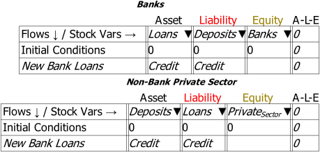
Figure 37 shows the absolute basic accounting for a Credit money system: banks create money by marking up both sides of their balance sheets. They add Credit dollars per year to Deposits, which are their Liabilities; and they add precisely the same sum to Loans, which are their Assets.
For the non-bank private sector, the act of borrowing also increases its Assets and Liabilities equally: Deposits, which are its Assets, rise by Credit dollars per year, and Loans, which are its Liabilities, rise by precisely the same amount. There is therefore no change in the net worth of either the Banking Sector, or the Non-Bank Private Sector from the creation of credit-money.
Figure 37: The fundamental accounting for Credit Money
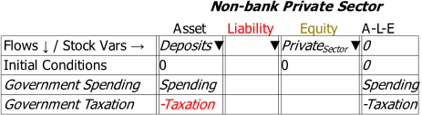
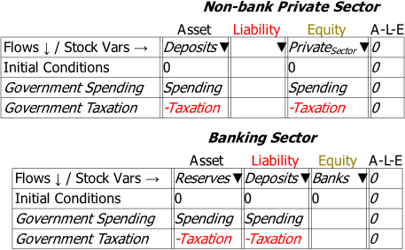
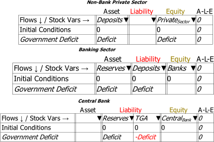
The Government’s role in money creation can be considered the same way, by modelling the two fundamental actions of governments: spending on the non-government private sector (either in the form of purchases or transfers), and taxation of the private sector.61F Figure 38 adds these to the Non-Bank Private Sector’s Godley Table in Figure 30, but without completing the double-entry.62F
Figure 38: Introducing Government Spending and Taxation without completing the double-entry
How should it be completed? I hope that it is obvious that the only way to complete this double-entry picture is that government spending increases the Equity—the net financial worth—of the non-bank private sector, while taxation reduces it.
This is shown in Figure 39. Government spending increases the net financial worth—the difference between financial assets and financial liabilities—of the private sector, and taxation reduces it.
Figure 39: The double-entry view of Government Spending and Taxation
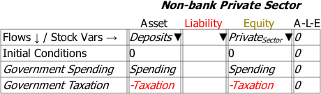
Figure 40 adds the Banking Sector’s Godley Table to the model, but also without completing the double-entry.
Figure 40: Government Spending and Taxation including the Banking Sector without completing the double-entry
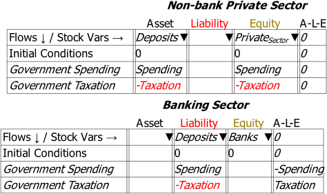
The only sensible way to complete this picture is to add an Asset which is increased by government spending (and reduced by taxation)—and this Asset is normally called “Reserves”.63F That is done in Figure 41 , which shows that government spending increases Reserves and Taxation reduces them.
Figure 41: Government Spending increases Reserves as well as Deposits—and taxation reduces them
At this point, several things should be obvious. Firstly, from the Liabilities side of the Banking system’s ledger, government spending creates money in the same way that new bank loans do, by increasing the Deposit accounts of the non-bank private sector. Similarly, taxation destroys money in the same way that the repayment of bank loans does, by reducing the Deposit accounts of the non-bank private sector.
Secondly, from the Assets side, net government spending—when government spending exceeds taxation—also increases the Assets of the banking sector, in the form of Reserves. This again is akin to how net loan growth—when new loans exceed the repayment of old loans—increases the Assets of the banking sector, in the form of Loans.
We can simplify the exposition of government money creation by defining the difference between government spending and taxation as the Deficit, and using that in future tables rather than using two rows for government spending and taxation respectively:
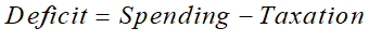
It follows therefore that a government Deficit—an excess of government spending over taxation—creates money for the Non-bank Private Sector, and creates Reserves for the Banking Sector, as shown in Figure 42.
Thirdly, since a Deficit adds to the Assets of the Non-bank Private Sector, without creating an offsetting Liability, as is the case with a bank loan, a Deficit increases the net worth—the Equity—of the Non-Bank Private Sector. Far from borrowing money from the private sector, as Neoclassical economists claim, the Deficit creates both money and net financial worth for the private sector.
Figure 42: A Government Deficit increases the net financial worth of the private sector
This is already a dramatically different assertion to the conventional wisdom that, as Mankiw puts it, a budget deficit is financed “by borrowing from the private sector” (Mankiw 2016, p. 555). And unlike the conventional wisdom, this assertion is logically sound. The only way the conventional wisdom could be correct would be if the Deficit had a negative impact on Deposit accounts. Then borrowing would occur as Deposits fell, another Asset of the non-bank private sector—”Loans to the Government”—rose. But in that case, government spending would have to decrease Deposits, and taxation would have to increase them! The conventional wisdom of economics, as is so often the case, is absurdly false.
Instead, just as bank lending creates money by increasing the banking sector’s Assets (Loans) and Liabilities (Deposits) simultaneously, a government deficit creates money by increasing the banking sector’s Assets (Reserves) and Liabilities (Deposits) simultaneously.
This leads to a general principle for money creation: since money is predominantly the Deposit accounts of the Non-Bank Private Sector, to create money, a financial operation must increase both the Assets and the Liabilities of the Banking Sector.64F
For banks, the process is easy—and this is why banks offer Deposit accounts in the first place. When a bank creates a loan, it marks up both sides of its balance sheet: it increases its Assets by adding to Loans, and it increases its Liabilities by adding to its customer Deposits. This is not possible for a Non-Bank Financial Institution: it can reallocate funds between its Assets, and gain when Assets increase in value, but it can’t increase the value of its Assets by its own operations. Banks can—so long as they can find willing borrowers.
The process of government money creation is more complicated than that of credit money creation, because the government can’t directly write up bank Assets and Liabilities. Instead, it has to increase a bank Asset—Reserves—after which banks will then allocate the same sums to the Deposit accounts of their customers.
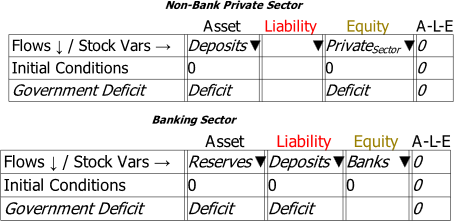
How are Reserves increased? To show that, we need to introduce a third Godley Table, that of the Central Bank. That is done in Figure 43, but without completing the double-entry logic.
Figure 43: Introducing the Central Bank without completing the double-entry
How do we balance that row? We could show this as negative equity for the Central Bank—if, as is the practice amongst many advocates of MMT (Modern Monetary Theory), we consolidated the Central Bank and the Treasury into one entity. But there’s no need to make that simplification with Minsky. We can, instead, show the financial sector in its realistic complexity, by adding another Liability of the Central Bank—the “deposit account” of the Treasury at the Central Bank. This is called the “Consolidated Revenue Fund” (CRF) in the UK, and the “Treasury General Account” in the USA (TGA). I use the American acronym in Figure 44.
Figure 44: The Central Bank with double-entry completed and the Treasury TGA introduced
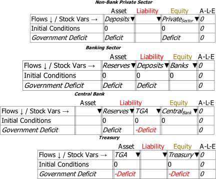
Reserves rise because of a transfer of funds from the TGA to Reserves. To show how these funds are generated, we need to add the Treasury’s Godley Table. That is done in Figure 45, again without completing the double-entry.
Figure 45: The Treasury Table introduced, without completing the double-entry
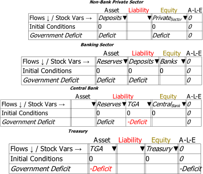
I hope it’s obvious that the only way to balance this line is the make the second entry in the Treasury’s Equity. That is done in Figure 46, which shows that the Treasury’s position is the exact opposite of the Non-Bank Private Sector’s: the positive Equity that the Deficit generates for the Private Sector is created by the Treasury going into identical negative Equity.
Figure 46: The completed basic picture of Government money creation
This simple picture appears unnatural to many people on first sight: what is the government doing, going into negative equity? Isn’t that a bad thing?
In fact, the government being in negative financial equity is the essence of fiat money. Banks create credit money by expanding their Assets and Liabilities equally; this results in a matching expansion of the non-bank private sector’s Liabilities and Assets. Governments create fiat money by going into negative Equity, which creates matching positive Equity for the non-bank private sector.
This can only work in the places in which a government’s liabilities are accepted as money, which define the locations in which it is the government. This is especially so for government operations on bank accounts. Sometimes, one country’s notes and coins are accepted as means of payment in another—you can sometimes use Euros to buy goods in Hungary, for example. But only the Hungarian government can directly add to Hungarian bank accounts by putting more Forints into them via government spending than it debits from them via taxation.
It is also of the essence of financial assets—claims on other entities—that the sum of all financial assets is zero. If one entity is in positive financial equity, then all other entities in an economy as in precisely the same negative financial equity with respect to it. What entity can sustain permanent negative financial equity? Not banks, because, by definition, banks must be in positive financial equity: a bank whose liquid liabilities exceed its liquid assets is bankrupt. The non-bank private sector can sustain negative financial equity, if its income is sufficient to service its debts, but it’s not a comfortable situation for individuals or companies to have liabilities that exceed their assets.
But a government, whose liabilities are money in its country, can always service its net negative financial position because it creates its own money. Finally, fiat money is backed by the extensive nonfinancial assets of a government: the unalienated land, the buildings, infrastructure, military, etc., of a nation state. There is, in other words, no problem with a government being in negative financial equity with respect to its own currency. It also means that, by running a sufficiently large deficit, it can ensure that both the Banking Sector and the Non-Bank Private Sector are in positive equity.
At this absolutely fundamental level then, net government spending does not involve borrowing from the private sector, and in fact it creates fiat money for the private sector. But what about government bonds? How do they change the picture? Don’t they mean that the government is borrowing from the private sector?
-
Government Bond Sales
One obvious consequence of the fundamental situation outlined above is that the Treasury’s account at the Central Bank must go negative. In and of itself, this isn’t a problem, since the Treasury and the Central Bank are both wings of the government, and in terms of where the Central Bank’s income is remitted, the Treasury is the effective owner of the Central Bank.65F It also has no implications for the solvency of the Central Bank, since the negative value of the TGA is precisely offset by the positive value of Reserves. Finally, as Central Banks themselves acknowledge (Bholat and Darbyshire 2016), unlike a private bank, it is not necessary for a Central Bank to be in positive equity.
However, virtually all governments have passed laws requiring the TGA to not go negative—and this is the real function of Treasury Bond sales. The upshot of these laws is that Treasuries are required to sell bonds equivalent in value to the deficit, plus interest on existing bonds.
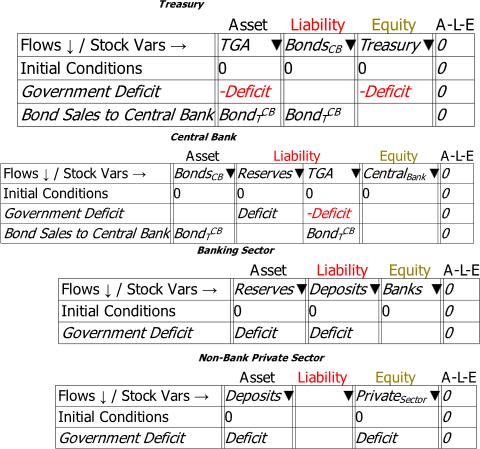
I’ll introduce government bond sales in the simplest possible way—as a sale of a bond to the Central Bank. This is in fact illegal in most countries, since they have also enacted laws that forbid the Central Bank from buying Bonds directly from the Treasury. But there is absolutely no practical impediment to this operation. It also has the side effect that interest payments are unnecessary: in most countries, the Treasury doesn’t pay interest on bonds owned by the Central Bank, and in those which do, the interest income is remitted back to the Treasury anyway. Therefore, interest payments on bonds—the cause of much angst in mainstream economics—can be omitted from the model.
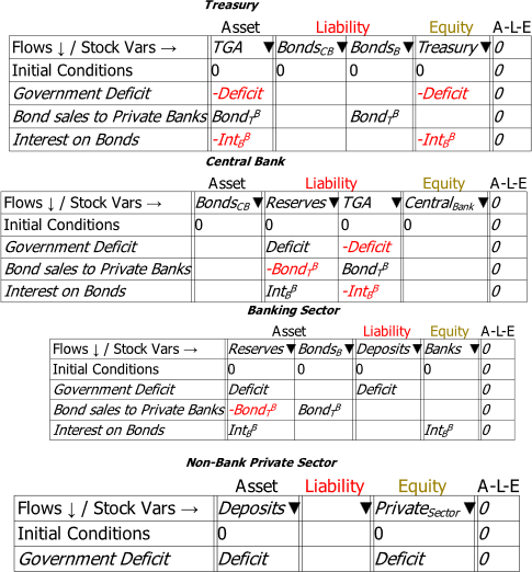
This hypothetical situation is shown in Figure 47. If the value of bonds sold by the Treasury to the Central Bank—shown as the flow —was equal to the Deficit, then the TGA would remain positive (or at least non-negative). This makes no practical difference to fiat money creation—that relies solely upon the Treasury going into negative equity—but is an aesthetic improvement on the situation shown in Figure 46, in that both Liability accounts of the Central Bank (Reserves and the TGA) would be positive. The Central Bank also has positive Assets, whereas in Figure 46 they are zero.
Figure 47: Treasury Bond Sales Direct to the Central Bank
The upshot of this arrangement for the Banking Sector is that the Asset that Deficits generate for it—Reserves—don’t normally earn income (by “normally” I mean “before the “Global Financial Crisis”). I suspect this detail—and not any desire to force prudence upon government money creation—is why most countries have made direct purchases of Treasury Bonds by the Central Bank illegal. Instead, these laws require the Treasury to sell Bonds to the private banks (and primary dealers),66F with the Central Bank then able to buy bonds from private banks in the “secondary market”.
The “magic” of this arrangement for the Banks is that the funds that private banks use to buy Bonds are created by the deficit itself—both the current deficit and the accumulation of past deficits known as government debt. Banks swap non-income-earning and non-tradeable Reserves for income-earning and tradeable Treasury Bonds. Since the Treasury does have to pay interest on bonds owned by the non-government sector, the act of selling Bonds to the Private Banks also necessitates paying interest on existing Bonds—which is otherwise known as existing Government debt. This generates an income stream for the Banking Sector.
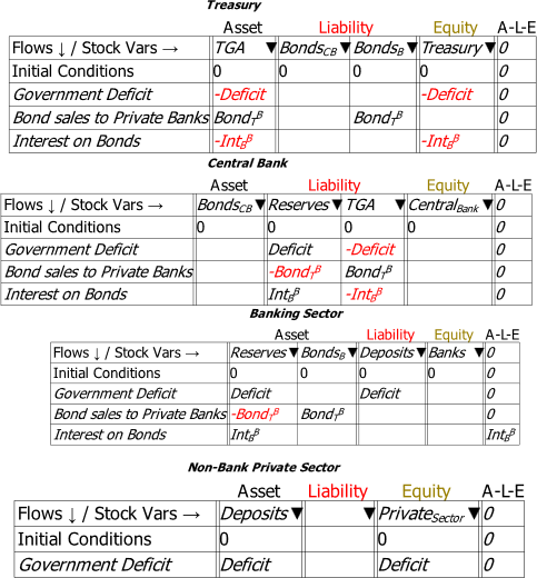
Figure 48 shows this legally required situation, without completing the double-entry details for the impact of interest on bonds for Private Banks. It should be obvious that this payment of interest adds to the net worth of the Banking Sector. And, just as the positive equity from the deficit for the non-bank private sector is created by the Treasury going into negative equity, the positive equity for the Banking Sector from government interest payments is also created by the Treasury going into negative equity.
Figure 48: Bond Sales to Private Banks, without completing the double-entry
A comparison of the above three Figures shows how absurd it is to describe the Treasury selling Bonds to the Banking Sector as the Treasury borrowing from the Banking Sector.
Neither arrangement is needed for the Treasury to create fiat money: the deficit alone does that, as Figure 46 shows, and it is financed by the Treasury going into negative equity, not by it selling Bonds to anyone. The only thing preventing Figure 46 from being the normal situation is a law requiring the TGA to not go into overdraft; if that law were repealed, there would be no need for Bond sales at all. Similarly, the only thing preventing Figure 47—direct Treasury bond sales to the Central Bank—is a law prohibiting it. These laws benefit the Banking Sector by letting it earn interest income on the Asset created for it by the Treasury, rather than (normally) not earning interest on Reserves.
Figure 49 completes the picture by showing interest on bonds as increasing the Equity of the Banks. It is then obvious that, just as the deficit creates net equity for the non-bank private sector, the payment of interest on bonds creates net equity for the banking sector.
Figure 49: Treasury Bond sales complicate the process, but don’t change the nature of fiat money
The final operation needed to complete the basic picture of government finances is the sale of Treasury Bonds by Banks to the non-bank private sector. Most of these sales are to Non-Bank Financial Institutions (NBFIs), but for simplicity I simply show this as a sale to the Non-Bank Private Sector in Figure 50. Once again, it would be ridiculous to describe this sale of a financial asset by the Banking Sector to the Non-bank Private Sector as “the government borrowing from the private sector”, but that’s how it’s described by Neoclassical economists.
Figure 50: Bond Sales to Non-Banks by Banks
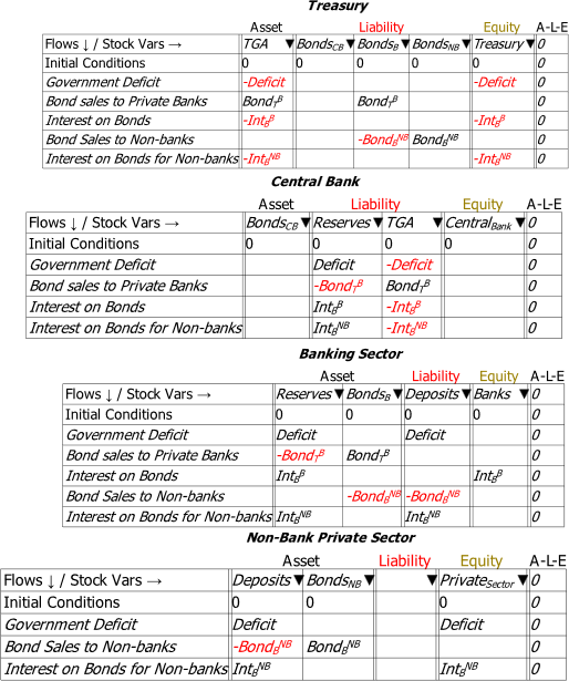
However, this operation is the only type of Bond sale that affects the quantity of money, and it reduces it rather than increasing it: Deposit accounts at banks fall, while the Non-bank Private Sector’s holdings of an income-earning Asset rise. The sale of Treasury Bonds by Banks to the Non-bank Private Sector—mainly to Non-Bank Financial Institutions (NBFIs)—thus destroys money.
We can now combine this model of fiat money creation—for that is what a Deficit actually is—with the model of credit money creation outlined in the previous chapter to show the real-world consequences of misunderstanding money creation. There is no better indication of the negative impact of mainstream misunderstandings about money than its role in causing the Great Depression.
-
Government Surpluses and the Roaring Twenties
Calvin Coolidge, who was President of the United States from 1923 till 1929, is lauded on the Whitehouse Presidents page for “his determination to preserve the old moral and economic precepts of frugality amid the material prosperity which many Americans were enjoying during the 1920s”.67F However, seen through the lens that Minsky provides into the dynamics of money creation, his governmental frugality contributed to the private excesses that caused the 1920s to be called “The Roaring Twenties”, and they also helped trigger the Great Depression.
Coolidge, of course, did not see it that way. He instead attributed the prosperity of the 1920s to the surplus he ran for all of his term. His final State of the Union Address68F lauded these surpluses as the cause of the prosperity of the 1920s:
No Congress of the United States ever assembled … has met with a more pleasing prospect than that which appears at the present time…
We have substituted for the vicious circle of increasing expenditures, increasing tax rates, and diminishing profits the charmed circle of diminishing expenditures, diminishing tax rates, and increasing profits.
Four times we have made a drastic revision of our internal revenue system… Each time the resulting stimulation to business has so increased taxable incomes and profits that a surplus has been produced. One-third of the national debt has been paid… It has been a method which has performed the seeming miracle of leaving a much greater percentage of earnings in the hands of the taxpayers ‘with scarcely any diminution of the Government revenue. That is constructive economy in the highest degree. It is the corner stone of prosperity. It should not fail to be continued.
This action began by the application of economy to public expenditure. If it is to be permanent, it must be made so by the repeated application of economy… Last June the estimates showed a threatened deficit for the current fiscal year of $94,000,000… The combination of economy and good times now indicates a surplus of about $37,000,000. This is a margin of less than 1 percent of our expenditures … It is necessary therefore … to refrain from new appropriations … otherwise, we shall reach the end of the year with the unthinkable result of an unbalanced budget. For the first time during my term of office we face that contingency. I am certain that the Congress would not pass and I should not feel warranted in approving legislation which would involve us in that financial disgrace. (Coolidge 1928. Emphasis added)
The data illustrates the success Coolidge’s determination to achieve a surplus every year: in every year of the Roaring Twenties, Receipts exceeded Outlays, and the amount averaged just below 1% of GDP every year—see Figure 51.
But, at the same time as Coolidge was “saving for a rainy day”, the private sector was borrowing like there was no tomorrow. And, from the accounting perspective provided in this Chapter, Coolidge was not saving money: he was instead destroying fiat money.
I cannot prove it, but I strongly suspect that the profligate borrowing and speculation of the 1920s was in part a response to Coolidge’s surpluses, which, as explained above, reduced the net financial worth of the non-government sector. This in turn would have motivated speculation by the non-bank private sector on the value of nonfinancial assets—primarily real estate and shares. As I explain shortly, this explosion of credit for nonfinancial assets drove up their prices, resulting in an amplifying feedback loop, in what has become known as a Ponzi Scheme (Zuckoff 2005), that drove firstly house prices (Vague 2019) and then share prices skyward. When the stock market scheme collapsed, it took the economy with it, and Coolidge’s much-treasured surpluses turned into deficits, which only partially compensated for the destruction of credit-based money that caused the Great Depression.
-
Government Surpluses and the Great Depression
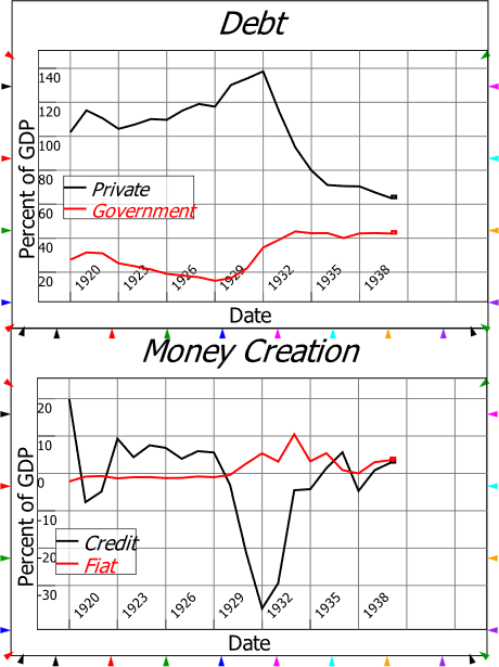
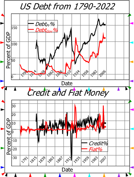
The data is stark: while Coolidge lauded his reduction of government debt from 30% to 15% of GDP, private debt rose from 100% to 140% of GDP at the same time. As he was—unwittingly—reducing fiat-backed money by 1% of GDP every year, the private sector was expanding credit-backed money by more than 5% of GDP each year. This, and not Coolidge’s surpluses, is what made the Twenties Roar—as I explain in the next section.
Even more staggering is the collapse in credit during the 1930s: credit swung from plus 5% of GDP in 1929 to minus 35% in 1932! Though the lack of a consistent time series on private debt makes the scale of the downturn in the 1930s questionable,69F the ratio of the collapse of credit in the 1930s to its expansion in the 1920s is not: the hit to aggregate demand from negative credit during the depths of the Great Depression was six times as large as the boost to aggregate demand from positive credit during the 1920s—see Figure 51.
Figure 51: Government and Private Debt and Money Creation 1920-4070F
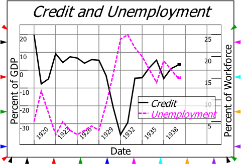
The relationship between credit and unemployment between 1920 and 1940 is the same as shown by Figure 35 for the period between 1990 and 2015: high credit means low unemployment and vice versa, because credit is the most volatile component of aggregate demand: see Figure 52.71F
Figure 52: Credit driving unemployment in the Roaring Twenties and Great Depression
In fact, the relationship is so significant that, when I first constructed a data set on debt back to 1790 using both modern Federal Reserve data and two Census data series (Census 1949, 1975)—see Figure 53—it alerted me to an economic crisis of which I was previously unaware: the “Panic of 1837”.
The event is so long back in history, and so precedes modern media—including both photographs and movies—that it has been largely forgotten. But in more contemporary accounts it was described as “an economic crisis so extreme as to erase all memories of previous financial disorders” (Roberts 2012, p. 24). Extant explanations of the crisis ascribe all manner of causes to it, but I identified it simply from the fact that it, like the “Great Recession” and the Great Depression, had an extended period of negative credit.
Like the Great Depression itself, this crisis was preceded by a period in which government debt was reduced substantially—in fact, all the way from 30 percent of GDP to zero. Private debt data before 1834 is unavailable, but it rose substantially from 1834 to 1837—from 78 to 99 percent of GDP—and it was in all likelihood rising before then, creating credit money. and masking the decline in fiat money caused by the deliberate reduction in government debt.
Then, as with the Great Depression, the Ponzi Schemes of those days collapsed, credit turned from very positive (18% of GDP in 1836) to very negative (minus 13% in 1841), and a serious economic and social crisis ensued.
The Great Depression remains the greatest crisis of all, with credit swinging from plus 5 to minus 35% of GDP: both the Panic of 1837 and the Global Financial Crisis pale in comparison. Bu the same characteristics apply: a period where the government was obsessed with reducing its debt levels, not realising that reducing government debt destroys fiat money, led to a period of private credit excess which masked the crisis until the Ponzi Scheme driving asset prices higher collapsed, triggering negative credit and an economic crisis.
Figure 53: Negative credit caused all three of America’s great crises
These inferences from the data can be analysed using a Minsky model of mixed fiat and credit money creation.
-
Modelling Coolidge’s Folly
A friend who once worked in marketing in Indonesia dines out on the story of when his firm won the Indonesian contract for the Kellogg Corporation. One of the Kellogg family came out to Jakarta, and in a meeting with his firm’s market team, he declared, in a broad Southern drawl, that “Ah think we’ll run with our usual campaign, that a bowl of Kellogg’s Cornflakes with milk an’ sugar gives ya 30% of yore daily nutritional needs”.72F
As the other executives nodded obediently, my friend put his hand up and asked “Excuse me sir, I don’t want to suggest this as an alternative campaign, I’m just curious. Can you tell us what the nutritional value of the bowl of Cornflakes is, without the milk and sugar?”
There was an embarrassingly long pregnant pause, after which the Kellogg family man drawled once more, “Well, ta be honest with ya sonny, nuthin’.”
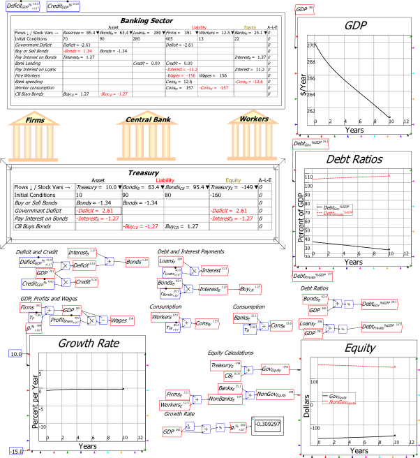
That anecdote neatly captures the value of running a government surplus with, and without, rising credit. With both a 1% of GDP surplus and 10% of GDP credit per year, Figure 54 shows the economy performs very nicely. GDP grows from 270 to 470 over ten years, the nominal growth rate is a healthy 5% per annum, and over the course of the decade, government debt drops by two thirds, from 33% to 11% of GDP. At the same time, private debt—that factor that Coolidge ignored, as have Neoclassical economists ever since 1870—rose from 104% to 135% of GDP. All these figures are close to what actually happened during the Roaring Twenties.
Figure 54: A mixed credit-fiat model with 1% government surplus and 10% credit

Figure 55 shows the same model with a 1% of GDP government surplus, but no credit. Just like the Kelloggs Cornflakes without the milk or sugar, there is no “nutritional value”. GDP falls from 270 to 260, and the annual rate of growth is minus 0.3%.
Figure 55: Coolidge’s 1% of GDP surplus with no credit
-
Isn’t this just MMT?
The analysis in this chapter is entirely derived from accounting identities, and it is also completely consistent with the analysis of “Modern Monetary Theory” as laid out by Stephanie Kelton in The Deficit Myth (Kelton 2020). What this chapter adds to MMT is firstly a proof that MMT’s analysis of government money creation is derived from a correct application of the rules of accounting, and is therefore better called “Modern Monetary Fact” as a result. Secondly it enables an integrated analysis of both fiat and credit money creation, which the MMT movement itself has not as yet provided, while mainstream Neoclassical economics ignores credit completely.
The ignored factor of credit was in fact responsible for the economic boom of the 1920s, and that credit, as many anecdotes, documentaries, novels and movies remind us, was showered upon the stock market. Everyone, from John D. Rockefeller to the bell hop, was buying shares on margin. With the rules of the day, $100 could buy $1000 worth of shares, thanks to a $900 margin loan from your friendly stockbroker. The appeal of margin debt, as your broker would confidently tell you, was that a 10% rise in the market would double your money: as your portfolio rose from $1000 to $1100, your equity rose from $100 to $200 (minus the trifling interest he charged you on your $900 debt to him, of course).
But what if it fell, you may have asked? Oh, no: “Stocks have reached a permanently high plateau”, as the great economist Irving Fisher assured everyone on October 16th, 1929 (Fisher 1929).73F Just sign on the dotted line. We must warn you that, if shares do fall 10%, then you are obliged to make up the lost $100 in a “margin call”, and all of your assets are available for liquidation to meet the call if you don’t have the ready cash. But don’t worry, that will never happen.
The scene was set for the greatest stock market crash in the history of capitalism.